

1. Introduction
Nonlinear evolution equations (NLEEs) constitute many fundamental models for describing intricate physical phenomena across diverse fields, including fluid dynamics, plasma physics, nonlinear optics, and Bose-Einstein condensates. In such systems, the interaction between dispersion and nonlinear terms always gives rise to nonlinear solutions with rich wave structures, notably solitons, breathers, and other localized waves [1-4]. Solitons are localized particle-like wave packets that can propagate over long distances while retaining their profile, amplitude and velocity. Breathers represent another class of localized nonlinear waves characterized by periodic oscillations in either temporal or spatial domains. Beyond individual wave structures, experimentally observed bound states, which comprise multiple coherent sub-pulses such as soliton molecules and breather molecules, have attracted significant interest [5-7]. Similarly to chemical molecules stabilized by strong bonds between atoms in chemical reactions, these bound states are the result of equilibrium between attractive and repulsive forces among the constituent sub-pulses. Theoretically, such bound-state structure can be derived by using the velocity resonance method, introduced by Lou [8]. This approach has been further extended to higher-dimensional systems, resulting in a broader variety of molecular wave patterns [9-11] and thereby substantially enriching nonlinear wave molecules.
Transformed waves refer to a specific category of nonlinear waves that emerge from the modulation of breathers [12-18]. In low-dimensional nonlinear Schrödinger-type equations, breathers may degenerate into solitons under special conditions [12-15]. Moreover, breather-to-soliton transitions have also been reported in high-dimensional spaces [16-18] and there notably these transformed waves feature time-varying characteristics. The aforementioned investigations, however, remain largely confined to constant-coefficient models, in which only simple wave structures can arise from the related fixed evolution mechanisms. This implies that in constant-coefficient systems there are inherent limitations to effectively modulate waveforms. In contrast, variable-coefficient systems offer greater physical fidelity by more accurately describing realistic physical phenomena and enabling the modulation of diverse waves [19-24]. Consequently, they may correspond to a much richer variety of wave patterns and more complex dynamical mechanisms. Through appropriate selection of inhomogeneous parameters within variable-coefficient systems, a number of novel wave phenomena have been discovered. For instance, in the variable-coefficient derivative nonlinear Schrödinger equation, non-autonomous breathers, periodic rogue waves, as well as new effects such as breather amplification and Talbot-like recurrence have been demonstrated [21]. For the non-autonomous Lenells-Fokas equation, higher-order periodic rogue waves, composite rogue waves (rogue wave pairs), and oscillating rogue waves have been obtained [22]. What is more, in higher-dimensional contexts, S-type breathers of the $(2+1)$-dimensional variable-coefficient Korteweg-de Vries equation and Y-shaped breathers in the $(2+1)$-dimensional variable-coefficient Kadomtsev-Petviashvili (KP) equation have been constructed via symmetry analysis [23] and bilinear KP hierarchy reduction method [24] respectively. These results indicate that in variable-coefficient systems the evolution of nonlinear waves can be controlled by well-chosen inhomogeneous coefficients and thus new wave structures can be obtained. Based on this special property, variable-coefficient systems may generate both time-invariant transformed waves and time-varying transformed waves through a strategic selection of coefficients.
In this paper, we aim to investigate the transition mechanisms, waves modulation, and interaction dynamics of nonlinear waves governed by the $(3+1)$-dimensional variable-coefficient Hirota bilinear system in fluids [25] 1 ) reduces to the $(3+1)$-dimensional Hirota bilinear system in [26-28], where the Bácklund transformation, rational-type solutions, rogue waves, and novel interaction solutions have been derived. Furthermore, imposing the additional condition $s_2 = 0$ on (1 ) simplifies the model to its $(2+1)$-dimensional version [29, 30], in which the integrability, solitons, invariant solutions, and interaction behavior have been investigated. For system (1 ), the Painlevé integrability, Lax pair, auto-Bácklund transformations, bilinear representations, and bilinear Bácklund transformations have been established in [25], while generalized higher-order rogue waves and Wronskian solutions have been constructed in [31]. Nevertheless, to the best of our knowledge, the behavior and properties of transformed waves within this system remain unexplored in the literature.
$\begin{align} & u_{yt}+g_1\left(t\right)\left(u_{xxxy}+6u_xu_y+3u_{xy}u+u_{xx}\left(3v+s_1\right)\right)+g_2\left(t\right)u_{yy}\nonumber\\ &\quad +s_2g_1\left(t\right)u_{zz} = 0,\nonumber\\ &\qquad\qquad\qquad\qquad\quad\;\;\,\, u_y = v_x, \end{align}$
where $u$ and $v$ are real differentiable functions of the variables $x$, $y$, $z$, and $t$, $g_1(t)$ and $g_2(t)$ are real differentiable functions of $t$, and $s_1$ and $s_2$ are nonzero real constants. The subscripts denote partial derivations with respect to the corresponding arguments. The Hirota bilinear system plays an important role in modeling nonlinear wave dynamics in various physical systems [25-31]. In fluid dynamics, it describes the dynamics of shallow water waves, internal ocean waves, and even tsunami waves. In nonlinear optics, it controls the propagation of optical solitons in planar waveguides and photonic lattices, helping in the study of spatiotemporal solitons and optical rogue waves. When $s_1 = 0$ and both $g_1(t)$ and $g_2(t)$ are taken to be arbitrary constants, system (The outline of this paper is as follows. Section 2 focuses on the construction of breather structures via the Hirota bilinear method. In section 3 , the breather-to-soliton transition conditions are established through characteristic line analysis. Subsequently, based on the phase difference analysis, various transformed waves with distinct properties are obtained. In section 4 , parabolic transformed waves are built up in virtue of parallel characteristic lines. Section 5 presents both long-lived and short-lived collisions between nonlinear waves. In section 6 , many wave molecules, including breather molecules, transformed wave-breather molecules, and transformed wave molecules, are constructed by employing the velocity resonance method. Finally, conclusions and remarks are contained in section 7 .
2. Structure of the breather solution of (1 )
We now construct the breather solution of system (1 ) via the Hirota bilinear method and analyze its constituent components. As a direct and effective approach, the Hirota bilinear method has been successfully used to solve numerous NLEEs, with a vast body of literature available for reference. Here, we list only a few of its more recent results. A large family of semi-rational solutions of the Maccari system has been obtained by combining the Hirota bilinear method with the KP hierarchy reduction method [32]. Moreover, the dark solitons, breathers, and resonant breathers have been presented via the Hirota bilinear method and KP-Toda reduction approach [33]. In addition, by using the Hirota bilinear method together with super Riemann theta functions, quasiperiodic wave solutions of supersymmetric integrable systems have been explicitly constructed [34].
Following [25], the bilinear form of system (1 ) takes the form of
$align*$
which admits the $N$-soliton solution $\begin{align} u = 2\left(\ln f_N\right)_{xx},\quad f_N = \sum_{\mu = 0,1} \exp\left(\sum_{j = 1}^N \mu_j \eta_j + \sum_{1\unicode{x2A7D} j \lt l\unicode{x2A7D} N}\mu_j\mu_l A_{jl}\right),\end{align}$
where $\begin{align} & \eta_j = k_j x + p_j y + m_j z-\omega_j \left(t\right) + \psi_j,\nonumber \\ &\exp\left(A_{jl}\right) \nonumber\\ &\quad = \frac{3k_jk_lp_jp_l\left(p_j-p_l\right)\left(k_j-k_l\right)-\left(p_jm_l-p_lm_j\right)^2s_2-\left(k_jp_l-k_lp_j\right)^2s_1}{3k_jk_lp_jp_l\left(p_j+p_l\right)\left(k_j+k_l\right)-\left(p_jm_l-p_lm_j\right)^2s_2-\left(k_jp_l-k_lp_j\right)^2s_1}, \end{align}$
with $align*$
Here $k_j$, $p_j$, $m_j$ are arbitrary constants, $\sum_{\mu = 0,1}$ stands for the summation over all possible combinations of $\mu_j, \mu_l = 0, 1$, $\sum_{1\unicode{x2A7D} j \lt l\unicode{x2A7D} N}$ is the summation over all distinct pairs $(j,l)$ satisfying $1\unicode{x2A7D} j \lt l\unicode{x2A7D} N$.For $N = 2$ in (2 ), we have the two-soliton solution 3 ). To obtain the breather solution for system (1 ), we set the parameters in (4 ) as paired-complexification of real parameters, namely 4 ) turns out to be 6 ) into (2 ), we obtain the breather solution 8 ) is related to those of its periodic wave component. The propagation velocities of the solitary wave component in the $x$-axis and $y$-axis are 7 ). We should point out that these characteristic lines often determine the propagation of the breather and force it to propagate as a robust, particle-like entity. And thus this also makes the characteristic lines highly significant for our subsequent research on the modulation of breathers.
$align$
where $\eta_1$, $\eta_2$ and $A_{12}$ are determined by ($\begin{align} &k_1 = k_2^* = a_1 + \mathrm{i}b_1 , \hspace{0.3cm} p_1 = p_2^* = c_1 + \mathrm{i}d_1, \hspace{0.3cm} m_1 = m_2^* = v_1 + \mathrm{i}w_1 , \nonumber\\ &\psi_1 = \psi_2^* = \delta_1 + \mathrm{i}\gamma_1, \hspace{0.3cm} \omega_1\left(t\right) = \omega_2^*\left(t\right) = \omega_{1\mathrm{R}}\left(t\right) + \mathrm{i}\omega_{1\mathrm{I}}\left(t\right),\nonumber\\ & \eta_1 = \eta_2^* = \eta_{1\mathrm{R}}+\mathrm{i}\eta_{1\mathrm{I}}, \end{align}$
where the $*$ indicates the complex conjugate, $a_1, b_1, c_1, d_1, v_1$, and $w_1$ are all nonzero real numbers, $\delta_1$ and $\gamma_1$ are both arbitrary real numbers. Then $f_2$ in ($\begin{align} f_2 & = 1 + 2\cos \eta_{1\mathrm{I}} \exp\left(\eta_{1\mathrm{R}}\right) + H_1 \exp\left(2\eta_{1\mathrm{R}}\right) \\ &\quad \sim 2\sqrt{H_1} \cosh\left( \eta_{1\mathrm{R}} + \frac{1}{2}\ln H_1\right) + 2 \cos \eta_{1\mathrm{I}}, \end{align}$
with $\begin{eqnarray} \begin{gathered} \eta_{1\mathrm{R}} = a_1 x + c_1 y + v_1 z - \omega_{1\mathrm{R}}\left(t\right) + \delta_1, \\ \eta_{1\mathrm{I}} = b_1 x + d_1 y + w_1 z - \omega_{1\mathrm{I}}\left(t\right) + \gamma_1, \\ H_1 = \frac{-3\left(a_1^2+b_1^2\right)\left(c_1^2+d_1^2\right)b_1d_1+\left(b_1^2s_1+w_1^2s_2\right)c_1^2+\left(a_1^2s_1+v_1^2s_2\right)d_1^2-2\left(a_1b_1s_1+v_1w_1s_2\right)c_1d_1}{3\left(a_1^2+b_1^2\right)\left(c_1^2+d_1^2\right)a_1c_1+\left(b_1^2s_1+w_1^2s_2\right)c_1^2+\left(a_1^2s_1+v_1^2s_2\right)d_1^2-2\left(a_1b_1s_1+v_1w_1s_2\right)c_1d_1}, \end{gathered}\end{eqnarray}$
in which $\begin{align} \omega_{1\mathrm{R}}\left(t\right) & = \int a_1\left(a_1^2 - 3b_1^2\right)\, g_1\left(t\right)\, \mathrm{d}t + \int c_1\, g_2\left(t\right)\, \mathrm{d}t\nonumber\\ &\quad + \frac{1}{c_1^2 + d_1^2} \int \left( s_1\left(a_1^2 c_1 + 2a_1 b_1 d_1 - b_1^2 c_1\right)\right.\nonumber\\ &\quad\left.+ s_2\left(v_1^2c_1 + 2v_1 w_1 d_1 - w_1^2 c_1\right)\right)\, g_1\left(t\right) \mathrm{d}t, \nonumber\\ \omega_{1\mathrm{I}}\left(t\right) & = \int b_1\left(3a_1^2 - b_1^2\right)\, g_1\left(t\right)\, \mathrm{d}t + \int d_1\, g_2\left(t\right)\, \mathrm{d}t \nonumber\\ &\quad + \frac{1}{c_1^2 + d_1^2} \int \left(s_1 \left(b_1^2 d_1 + 2a_1 b_1 c_1 - a_1^2 d_1\right)\right.\nonumber\\ &\quad\left.+ s_2\left(w_1^2d_1 + 2v_1 w_1 c_1 - v_1^2d_1\right) \right)\, g_1\left(t\right) \mathrm{d}t. \end{align}$
By substituting ($\begin{align} u& = \frac{2\left(a_1^2\sqrt{H_1}\cosh\Omega-b_1^2\cos \eta_{1\mathrm{I}}\right)}{\sqrt{H_1}\cosh\Omega+\cos \eta_{1\mathrm{I}}} \nonumber\\ &\quad -\frac{2\left(a_1\sqrt{H_1}\sinh\Omega-b_1\sin \eta_{1\mathrm{I}}\right)^2}{\left(\sqrt{H_1}\cosh\Omega+\cos \eta_{1\mathrm{I}}\right)^2}, \end{align}$
with $\Omega = \eta_{1\mathrm{R}}+\frac{1}{2}\ln H_1$. The existence of both hyperbolic and trigonometric functions in this expression clearly shows that the breather solution can be regarded as a nonlinear superposition of solitary wave and periodic wave components, which simultaneously determine the fundamental properties of the breather. Hyperbolic functions $(\cosh\Omega,\sinh\Omega)$ determine its locality and, in the meantime, trigonometric functions $(\cos \eta_{1\mathrm{I}},\sin \eta_{1\mathrm{I}})$ imply its periodicity. The formation of peaks and troughs of the breather ($align*$
and the propagation velocities of the periodic wave component in the $x$-axis and $y$-axis are $align*$
where the superscripts ${s}$ and ${p}$ represent the solitary wave and the periodic wave, respectively. Moreover, the characteristic line of the solitary wave component is $\begin{align} L_{11}:\ \ \eta_{1\mathrm{R}}+\frac{1}{2}\ln H_1 = 0,\end{align}$
and the characteristic line of periodic wave component reads as $\begin{align} L_{12}:\ \ \eta_{1\mathrm{I}} = 0,\end{align}$
where $\eta_{1\mathrm{R}}$, $\eta_{1\mathrm{I}}$, and $H_1$ are given in (The structure of the breather (8 ) is shown in figure 1. Figures 1(a) and (b) depict the spatial structure and contour of the breather at $t = 0$, where the characteristic lines are $L_{11}:\ y = -0.4x - 1.468t^3 + 0.5t^2 - 0.456\,526\,5722$ and $L_{12}:\ y = 2x - 0.206\,666\,6666t^3 + 0.5t^2$ and they intersect at angle $\theta$. What is more, characteristic lines at both $t = 0$ and $t = 3$ are shown in figure 1(c), in which we notice that the included angles $\theta$ and slopes remain constant over time. As mentioned above, the invariant, locked structure of characteristic lines is the fundamental reason why the shape and amplitude of the breather are maintained throughout its propagation.
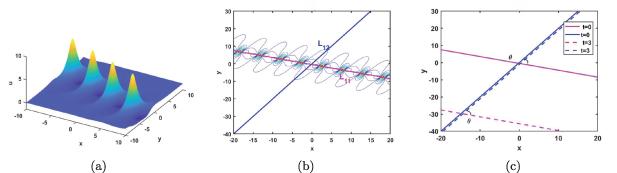
Figure 1. Breather with $s_1 = s_2 = 1$, $a_1 = 0.2$, $b_1 = 1$, $c_1 = 0.5$, $d_1 = -0.5$, $v_1 = 1$, $w_1 = 0.5$, $g_1 = t^2$, $g_2 = t$. (a) Spatial structure at $t = 0$. (b) The contour plot at $t = 0$. (c) The characteristic lines at $t = 0$ and $t = 3$. |
3. Modulation of waveforms for transformed waves
In this section, we begin by investigating the formation mechanism of transformed waves in equation (1 ), through an analysis of the positional relationship between the two characteristic lines $L_{11}$ and $L_{12}$ of the solitary wave and periodic wave components. On the basis of phase shift analysis, the phase difference between the two wave components is derived. Subsequently, several examples of shape-preserving and shape-changing transformed waves are constructed by appropriately selecting inhomogeneous coefficients in (1 ).
The positional relationship between the characteristic lines $L_{11}$ and $L_{12}$ always determines the wave state. More specifically, when the two characteristic lines intersect, the wave remains in a breather state. In contrast, when they are parallel, a number of types of transformed waves emerge. Meanwhile, the interaction between the solitary wave and periodic wave components leads to the localized oscillatory characteristic observed in both breathers and transformed waves. Figure 2 provides an intuitive illustration of these nonlinear superposition mechanisms, where 'P $\rightarrow$' and 'S $\rightarrow$' denote the propagation directions of the periodic wave and the solitary wave, respectively. In figure 2(a), the crossed superposition of the solitary and periodic waves yields a breather, while in figure 2(b), their parallel superposition produces a transformed wave.
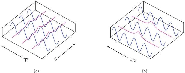
Figure 2. The superposition modes. (a) The breather: the crossed superposition mode. (b) The transformed wave: the parallel superposition mode. |
In the $(x,y)$ plane, based on this property and following (9 ) and (10 ), the transition conditions of breather-to-soliton can be derived, being
$\begin{equation} \left| \begin{array}{cc} a_1 & b_1 \\ c_1 & d_1 \\ \end{array} \right| = 0.\end{equation}$
Similarly, in the $(x, z)$ and $(y, z)$ planes, the conditions for the breather-to-soliton transition take the form of $\begin{equation*} \left| \begin{array}{cc} a_1 & b_1 \\ v_1 & w_1 \\ \end{array} \right| = 0, \quad \left| \begin{array}{cc} c_1 & d_1 \\ v_1 & w_1 \\ \end{array} \right| = 0,\end{equation*}$
respectively. For brevity, here we focus only on the $(x, y)$ plane for an in-depth analysis, and the corresponding results for the other two planes can be derived analogously.In the $(x, y)$ plane, when the transition condition (11 ) is satisfied, the breather solution given by equation (8 ) turns out to be a transformed wave: 7 ) under the transition condition.
$\begin{align} u& = \frac{2\left(a_1^2\sqrt{\widetilde{H}_1}\cosh\widetilde{\Omega}-b_1^2\cos \widetilde{\eta}_{1\mathrm{I}}\right)}{\sqrt{\widetilde{H}_1}\cosh\widetilde{\Omega}+\cos \widetilde{\eta}_{1\mathrm{I}}} \nonumber\\ &\quad -\frac{2\left(a_1\sqrt{\widetilde{H}_1}\sinh\widetilde{\Omega}-b_1\sin \widetilde{\eta}_{1\mathrm{I}}\right)^2}{\left(\sqrt{\widetilde{H}_1}\cosh\widetilde{\Omega}+\cos \widetilde{\eta}_{1\mathrm{I}}\right)^2}, \end{align}$
where $\widetilde{H}_1$, $\widetilde{\Omega}$ and $\widetilde{\eta}_{1\mathrm{I}}$ represent the corresponding quantities in (The variable-coefficient model investigated here differs fundamentally from constant-coefficient models. In a constant-coefficient system, the phase difference between the solitary and periodic wave components, arising from their relative velocity, continuously alters the superposition region and therefore causes the waveform of the transformed wave to vary over time [16-18]. In contrast, the presence of inhomogeneous coefficients in a variable-coefficient model allows the velocities of the wave components to be actively adjusted. Consequently, by fixing the phase differences, one can modulate the waveforms of the transformed waves. We now proceed to analyze the phase differences between the solitary and periodic wave components.
From (7 ), the phase shifts of the solitary wave component $(\phi_{s})$ and periodic wave component $(\phi_{p})$ are obtained as:
$\begin{align*} \phi_{s} = -\omega_{1\mathrm{R}}\left(t\right) +\frac{1}{2} \ln H_1 , \hspace{1cm} \phi_{p} = -\omega_{1\mathrm{I}}\left(t\right),\end{align*}$
yielding the phase difference $align*$
between the two components therein. To modulate the waveforms of transformed waves in a variable-coefficient model while preserving waveforms, the phase difference must remain constant throughout the evolution, i.e. $align$
Taking an M-shaped soliton as an example, this time-invariant property is exhibited in figure 3. Figures 3(a)-(c) display its spatial structures at $t = -1,0,1$ respectively. Figure 3(d) shows its cross-sectional profiles, confirming that the transformed wave maintains its shape during propagation. Figure 3(e) presents the distribution of characteristic lines at different time instances, where the distances between the characteristic lines keep invariant over time, thereby further revealing the underlying shape-preserved mechanism of transformed waves.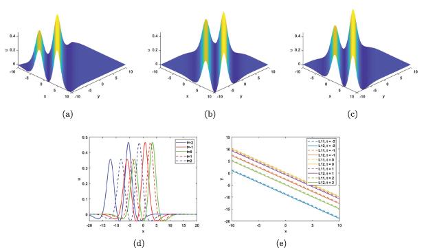
Figure 3. Spatial structure of the shape-preserving M-shaped soliton with $s_1 = s_2 = 1$, $a_1 = b_1 = c_1 = d_1 = 0.6$, $v_1 = 1.297\,923\,628$, $w_1 = -1.079\,910\,063$, $g_1 = t$, $g_2 = t^2$. (a) $t = -1$. (b) $t = 0$. (c) $t = 1$. (d) The cross-sectional profiles at different time instants. (e) The characteristic line of the solitary wave $L_{11}:y = -x-1.446\,723\,316 t^2 +0.333\,333\,3333t^3+0.470\,544\,9535$ (solid line) and the periodic wave $L_{12}:y = -x-1.446\,723\,31t^2+0.333\,333\,3333 t^3$ (dotted line). |
In short, these results indicate that a proper choice of inhomogeneous coefficients can adjust the phase difference to satisfy condition (13 ), thereby producing a shape-preserving transformed wave.
On the contrary, when condition (13 ) is not met, the resulting transformed waves exhibit time-varying property, that is, their shapes evolve over time, which is a typical behavior in high-dimensional constant-coefficient systems. As shown in figure 4, appropriately chosen parameters can generate shape-changing transformed waves. For instance, figures 4(a1), (b1) and (a2), (b2) depict the spatial structures of a shape-changing M-shaped transformed wave at different time instants under distinct inhomogeneous coefficients. To highlight the time-varying property of the transformed wave, several cross-sectional profiles are also provided. Figures 4(c1) and (c2) illustrate how the waveform changes at different times under the same inhomogeneous coefficients, while figures 4(a3) and (b3) reveal the influence of different inhomogeneous coefficients on the waveform at the same instant.
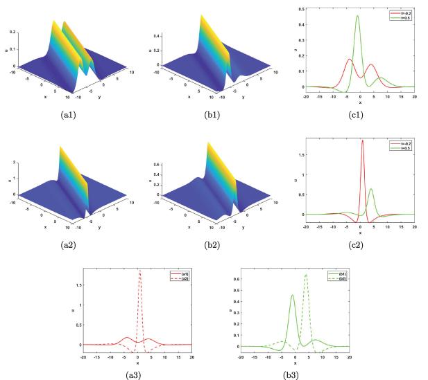
Figure 4. The shape-changing M-shaped transformed wave with parameters $s_1 = 3$, $s_2 = 2$, $a_1 = 0.4$, $b_1 = 0.3$, $c_1 = 0.8$, $d_1 = 0.6$, $v_1 = 1$, $w_1 = 2$ for two cases: (i) $g_1 = t$, $g_2 = 1$ and (ii) $g_1 = \cos t$, $g_2 = 1$. For case (i), (a1) and (b1) show the transformed wave at $t = -0.2$ and $t = 0.5$, for case (ii), (a2) and (b2) show the transformed wave at $t = -0.2$ and $t = 0.5$. (c1) and (c2) display the cross-sectional profiles of (a1), (b1) and (a2), (b2). (a3) and (b3) compare the profiles of (a1), (a2) and (b1), (b2). |
4. Parabolic transformed waves in the $(x, t)$ plane
To facilitate the intuitive visualization of the temporal evolution of waveforms, we now concentrate our analysis on the systematic construction of parabolic transformed waves through characteristic line analysis in the $(x, t)$ plane.
With the inhomogeneous parameters $g_1 = t$, $g_2 = t+1$ and with fixed values $s_1 = s_2 = 1$, $y = 0$ and $z = 0$, in view of (9 ) and (10 ), the characteristic lines for the solitary wave and periodic wave components are
$\begin{eqnarray} \begin{aligned} &L_1: \qquad M_1x + N_1t + Q_1 t^2 -\left(c_1^2 +d_1^2\right)\ln H_1 = 0, \\ &L_2: \qquad M_2x +N_2t +Q_2 t^2 = 0, \end{aligned}\end{eqnarray}$
with $\begin{align} M_1& = -2a_1\left(c_1^2 +d_1^2\right),\hspace{0.3cm}N_1 = 2c_1\left(c_1^2 +d_1^2\right), \nonumber\\ Q_1& = a_1^3\left(c_1^2 + d_1^2\right) - 3a_1b_1^2\left(c_1^2 +d_1^2\right) \nonumber\\ &\quad + c_1\left(a_1^2 -b_1^2 + c_1^2 + d_1^2 + v_1^2 - w_1^2\right) +2a_1b_1d_1+ 2d_1v_1w_1, \nonumber\\ M_2& = -2b_1\left(c_1^2 +d_1^2\right),\hspace{0.3cm}N_2 = 2d_1\left(c_1^2 +d_1^2\right), \nonumber\\ Q_2& = - b_1^3\left(c_1^2 + d_1^2\right)+3a_1^2b_1\left(c_1^2 + d_1^2\right) \nonumber\\ &\quad - d_1\left(a_1^2 -b_1^2 - c_1^2 - d_1^2 +v_1^2 -w_1^2\right)+2a_1b_1c_1+ 2c_1v_1w_1. \end{align}$
As established in section 4 , transformed waves emerge if and only if these characteristic lines are parallel. Therefore, on the $(x, t)$ plane, the parallelism criterion
$\begin{equation} \left| \begin{array}{cc} M_1 & N_1 \\ M_2 & N_2 \\ \end{array} \right| = \left| \begin{array}{cc} N_1 & Q_1 \\ N_2 & Q_2 \\ \end{array} \right|,\end{equation}$
guarantees the generation of transformed waves. From the perspective of the nonlinear superposition mechanism, because the periodic wave component mainly affects the envelope region of the solitary wave component, the oscillatory region of the transformed wave is localized. Note that the wave number ratio $\frac{a_1}{b_1}$ plays a key role in controlling the waveform. When this ratio is much greater than $1$, the wave can be regarded as the superposition of a solitary wave and an extremely low-frequency periodic wave. In this case, the periodic component has almost no effect on the solitary wave, leading to the formation of a quasi-soliton. As the ratio approaches $1$, the frequency of the periodic wave increases, causing oscillations to appear in the envelope of the solitary wave. Consequently, it evolves into an M-shaped soliton with two peaks and one trough. When the ratio becomes less than $1$, the effect of the periodic wave on the solitary wave becomes stronger, the number of peaks increases, and multi-peak solitons are eventually formed.Based on above analysis, various types of parabolic transformed waves can be generated by properly adjusting the ratio $\frac{a_1}{b_1}$. Several representative examples are illustrated in figures 5-7, which correspond to a quasi-soliton, an M-shaped soliton and a multi-peak soliton with $\frac{a_1}{b_1} = 20, 1, 0.33$ respectively. From these results, it can be clearly observed that although the characteristic lines remain parallel in all cases, the waveform evolves significantly as the ratio $\frac{a_1}{b_1}$ decreases from $20$ to $0.33$. Specifically, the number of wave peaks gradually increases, successively yielding a sequence of different structures, from a quasi-soliton, to an M-shaped soliton, and finally to a multi-peak M-shaped soliton.
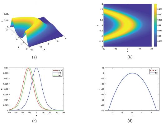
Figure 5. The parabolic quasi-soliton with $a_1 = 0.2$, $b_1 = 0.01$, $c_1 = 0.2$, $d_1 = 0.01$, $v_1 = -0.050\,080\,199\,68$, $w_1 = 1$. (a) Spatial structure. (b) The density plot. (c) The waveforms at $t = -1, 0, 1$. (d) The characteristic lines of solitary wave ($L_1:\ 0.2x + 2.296\,029\,984t^2 $ $- 0.2t - 0.002\,400\,239\,19 = 0$ in blue) and periodic wave ($L_2:\ 0.01x + 0.114\,801\,4992t^2 - 0.01t = 0$ in red). |
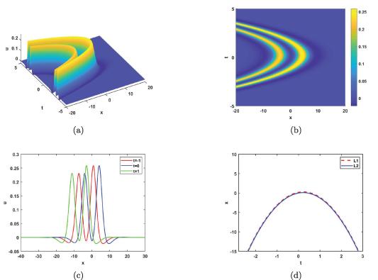
Figure 6. The parabolic M-shaped soliton with $a_1 = 0.4$, $b_1 = 0.4$, $c_1 = 0.4$, $d_1 = 0.4$, $v_1 = -1.049\,952\,380$, $w_1 = 1$. (a) Spatial structure. (b) The density plot. (c) The waveforms at $t = -1, 0, 1$. (d) The characteristic lines of solitary wave ($L_1:\ 0.4x + 0.912\,440\,4750t^2 $ $- 0.4t - 0.073\,233\,381\,60$ in blue) and periodic wave ($L_2:\ 0.4x + 0.912\,440\,4750t^2 - 0.4t$ in red). |
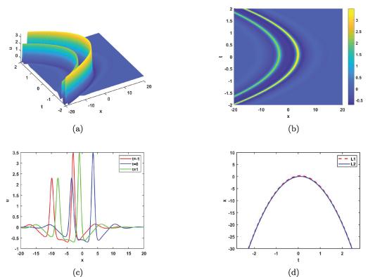
Figure 7. The parabolic multi-peak soliton with $a_1 = 0.2$, $b_1 = 0.6$, $c_1 = 0.2$, $d_1 = 0.6$, $v_1 = -3.047\,328\,018$, $w_1 = 1$. (a) Spatial structure. (b) The density plot. (c) The waveforms at $t = -1, 0, 1$. (d) The characteristic lines of solitary wave ($L_1:\ 0.2x + 0.998\,996\,0060t^2 $ $- 0.4t - 0.005\,969\,036\,08 = 0$ in blue) and periodic wave ($L_2:\ 0.1x + 0.499\,498\,0030t^2 - 0.2t = 0$ in red). |
5. Long- and short-lived collision between nonlinear waves
Here we study the collision mechanisms of two nonlinear waves governed by (1 ). To this aim, we need to consider the four-soliton solution defined by (2 ), under two sets of complex conjugate parameters.
In the case of $N = 4$, adopting the parameters $k_1, p_1, m_1$ and $\phi_1$ as defined in (5 ) and setting 2 ), we arrive at 7 ), $H_3$ given by (7 ) but under the parameter substitution $(a_1,b_1,c_1,d_1,v_1,w_1)\mapsto(a_3,b_3,c_3,d_3,v_3,w_3)$, and $H_{1\mathrm{R}} = \mathrm{Re}\left( \mathrm{e}^{A_{13}} \right)$, $H_{1\mathrm{I}} = \mathrm{Im}\left( \mathrm{e}^{A_{13}} \right)$, $H_{3\mathrm{R}} = \mathrm{Re}\left( \mathrm{e}^{A_{14}} \right)$, $H_{3\mathrm{I}} = \mathrm{Im}\left( \mathrm{e}^{A_{14}} \right)$. To (1 ), substituting (17 ) into (2 ) yields a standard second-order breather solution consisting of two breather components as shown in figure 8, where figure 8(a) presents the collision of the two breathers and figure 8(b) depicts the associated phase shift induced by the collision. Different from the first-order breather solution (8 ), the second-order breather solution has two sets of characteristic lines. In what follows, for convenience of discussion we use ($L_{11}, L_{12}$), ($L_{31}, L_{32}$) to denote the characteristic lines to the two breathers components, namely 11 ) and
$\begin{eqnarray*} \begin{aligned} &k_3 = k_4^* = a_3 + \mathrm{i}b_3 , \hspace{0.3cm}p_3 = p_4^* = c_3 + \mathrm{i}d_3 , \hspace{0.3cm}m_3 = m_4^* = v_3 + \mathrm{i}w_3 , \hspace{0.3cm} \\ &\psi_3 = \psi_4^* = \delta_3 + \mathrm{i}\gamma_3 , \hspace{0.3cm} \omega_3\left(t\right) = \omega_4^*\left(t\right) = \omega_{3\mathrm{R}}\left(t\right) + \mathrm{i}\omega_{3\mathrm{I}}\left(t\right) ,\nonumber\\ & \eta_3 = \eta_4^* = \eta_{3\mathrm{R}}+\mathrm{i}\eta_{3\mathrm{I}}, \end{aligned}\end{eqnarray*}$
in view of ($\begin{align} f_4 &= 1+2\mathrm{e}^{\eta_{1\mathrm{R}}}\cos \eta_{1\mathrm{I}}+H_1\mathrm{e}^{2\eta_{1\mathrm{R}}}+2\mathrm{e}^{\eta_{3\mathrm{R}}}\cos\eta_{3\mathrm{I}}+H_3\mathrm{e}^{2\eta_{3\mathrm{R}}}\nonumber\\ &\quad+H_1\mathrm{e}^{2\eta_{1\mathrm{R}}+\eta_{3\mathrm{R}}}\left(\left(H_{1\mathrm{R}}H_{3\mathrm{R}}+H_{1\mathrm{I}}H_{3\mathrm{I}}\right)\cos\eta_{3\mathrm{I}}\right.\nonumber\\ &\quad\left.-\left(H_{1\mathrm{I}}H_{3\mathrm{R}}-H_{1\mathrm{R}}H_{3\mathrm{I}}\right)\sin \eta_{3\mathrm{I}}\right) \nonumber\\ &\quad+H_3\mathrm{e}^{\eta_{1\mathrm{R}}+2\eta_{3\mathrm{R}}}\left(\left(H_{1\mathrm{R}}H_{3\mathrm{R}}-H_{1\mathrm{I}}H_{3\mathrm{I}}\right)\cos \eta_{1\mathrm{I}}\right.\nonumber\\ &\quad\left.-\left(H_{1\mathrm{I}}H_{3\mathrm{R}}+H_{1\mathrm{R}}H_{3\mathrm{I}}\right)\sin \eta_{1\mathrm{I}}\right) \nonumber\\ &\quad+2\mathrm{e}^{\eta_{1\mathrm{R}}+\eta_{3\mathrm{R}}}\left(H_{1\mathrm{R}}\cos\left(\eta_{1\mathrm{I}}\!+\!\eta_{3\mathrm{I}}\right)\!-\! H_{1\mathrm{I}}\sin\left(\eta_{1\mathrm{I}}\!+\!\eta_{3\mathrm{I}}\right)\right.\nonumber\\ &\quad\left.\!+\!H_{3\mathrm{R}}\cos\left(\eta_{1\mathrm{I}}\!-\!\eta_{3\mathrm{I}}\right)\!-\!H_{3\mathrm{I}}\sin\left(\eta_{1\mathrm{I}}\!-\!\eta_{3\mathrm{I}}\right)\right) \nonumber\\ &\quad+H_1H_3\mathrm{e}^{2\eta_{1\mathrm{R}}+2\eta_{3\mathrm{R}}}\left(H_{1\mathrm{R}}^2+H_{1\mathrm{I}}^2\right)\left(H_{3\mathrm{R}}^2+H_{3\mathrm{I}}^2\right), \end{align}$
with $H_1$ defined by ($\begin{eqnarray} \begin{aligned} &L_{j1}:\qquad a_j x + c_j y - \omega _{j\mathrm{R}}\left(t\right)+\frac{1}{2}\ln H_j = 0, \\ &L_{j2}:\qquad b_j x + d_j y - \omega _{j\mathrm{I}}\left(t\right) = 0, \end{aligned}\end{eqnarray}$
for $j = 1,3$. And for the two breathers, the correspondingly transition conditions are ($\begin{equation} \left| \begin{array}{cc} a_3 & b_3 \\ c_3 & d_3 \\ \end{array} \right| = 0,\end{equation}$
respectively.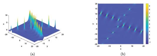
Figure 8. Second-order breather at $t = 0$ with $s_1 = s_2 = 1$, $a_1 = 0.2$, $b_1 = 1$, $c_1 = 0.5$, $d_1 = -0.5$, $v_1 = 1$, $w_1 = 0.5$, $\delta_1 = \gamma_1 = 0$, $a_3 = -0.5$, $b_3 = 0.1$, $c_3 = 0.4$, $d_3 = v_3 = 1$, $w_3 = 0.5$, $\delta_3 = \gamma_3 = 0$, $g_1 = g_2 = t$. (a) Spatial structure. (b) The density plot. |
Based on the second-order breather solution, one can obtain diverse types of collision modes. According to the analysis in section 3 , a breather transforms into a soliton when its transition condition is satisfied. As a result, when both breathers satisfy their respective transition conditions, a full-transition occurs, with each breather converting into a soliton, which is illustrated in figures 9 and 10. The interaction in figure 9 is a long-lived collision, featured by a sustained interaction period where the characteristic lines of the two waves intersect, as shown in figure 9(c). Figure 9(b) reveals a significant amplitude change in one of the transformed waves after the collision, indicating that the collisions directly affect wave amplitudes. In sharp contrast with the long-lived collision in figure 9, figure 10 demonstrates a short-lived collision, in which the characteristic lines of the two waves remain parallel. The evolution at three different instants is shown in figures 10(a)-(c). At $t = -1$, the higher-amplitude transformed wave is located to the left of the lower-amplitude one. At $t = 0$, they collide, combining into a single M-shaped wave. At $t = 0.5$, the higher-amplitude wave has overtaken the other and continues to propagate ahead. For these time instants, the corresponding characteristic lines, shown in figures 10(d)-(f) validate this short-lived collision, the red solid line gradually approaches and eventually surpasses the blue one, during the evolution.
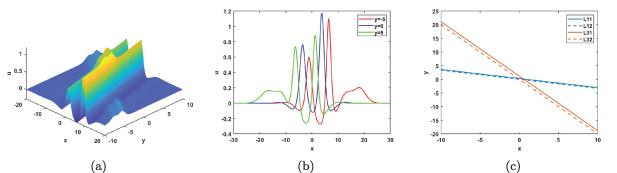
Figure 9. The long-lived collision of two transformed waves at $t = 0$ with $s_1 = 1$, $s_2 = 2$, $a_1 = 0.5$, $b_1 = 0.2$, $c_1 = 1.5$, $d_1 = 0.6$, $v_1 = w_1 = 1$, $\delta_1 = \gamma_1 = 0$, $a_3 = 0.4$, $b_3 = 0.6$, $c_3 = 0.2$, $d_3 = 0.3$, $v_3 = 0.5$, $w_2 = 3$, $\delta_3 = \gamma_3 = 0$, $g_1 = g_2 = t$. (a) Spatial structure. (b) Cross-sectional plots at $y = -5, 0, 5$. (c) Two sets of characteristic lines ($L_{11}:\ y = - 0.333\,333\,3333x + 0.883\,735\,6320t^2+0.300\,870\,8717$, $L_{12}:\ y = -0.333\,333\,3333x + 2.589\,597\,702t^2$ in red, and $L_{31}:\ y = - 2x - 4.189\,230\,770t^2+1.168\,474\,823,\,\,\,L_{32}:\ y = -2 x + 41.722$ $\,564\,10t^2$ in blue). |
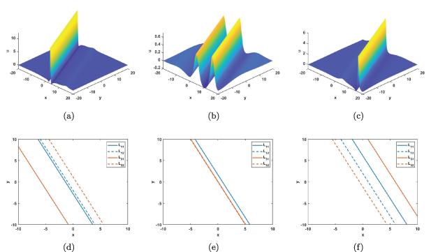
Figure 10. The short-lived collision of two transformed waves with $s_1 = s_2 = 1$, $a_1 = 0.2$, $b_1 = 0.4$, $c_1 = 0.1$, $d_1 = 0.2$, $v_1 = w_1 = 1$, $\delta_1 = \gamma_1 = 0$, $a_3 = 0.3$, $b_3 = 0.4$, $c_3 = 0.15$, $d_3 = 0.2$, $v_3 = 3$, $w_3 = 1$, $\delta_3 = -5$, $\gamma_3 = 0$, $g_1 = t$, $g_2 = 2t$. (a)-(c) Spatial structures at $t = -1, 0, 0.5$. (d)-(f) Two sets of characteristic lines of (a)-(c) ($L_{11}:\ y = - 2x + 27.706\,666\,67t^3 + 2t+1.663\,528\,769$, $L_{12}:\ y = -2x + 7.973\,333\,330t^3 + 2t$ in red, and $L_{31}:\ y = - 2x + 86.406\,666\,67t^3 + 2t+0.096\,849\,733\,47,\,\,L_{32}:\ y = -2x - 17.260\,$ $ 000\,00t^3+ 2t$ in blue). |
6. Molecular waves
As mentioned in the introduction, the velocity resonance method has been widely adopted in the construction of molecules for many nonlinear models. The essence of this method is to generate bound-state structures by controlling the propagation velocities of involved waves to satisfy specific resonance conditions. In this section, we employ the velocity resonance method to construct molecular waves from the two breathers associated with the second-order breather solution obtained in section 5 via (2 ) and (17 ). For these two breathers, the resonance conditions read as 11 ), (13 ), (19 ), and (20 ) are met partially or completely, distinct molecular waves, including breather molecules, transformed wave-breather molecules and transformed wave molecules, emerge.
$\begin{align} L_{11}\,\, /\!\!/\,\, L_{31}, \boldsymbol{v}_1 = \boldsymbol{v}_3, \end{align}$
with $\begin{align*} \boldsymbol{v}_j = \left(\frac{\omega_{j\mathrm{R}}\left(t\right)}{a_j},\frac{\omega_{j\mathrm{R}}\left(t\right)}{c_j}\right)^\mathsf{T},\qquad j = 1,3, \end{align*}$
being velocities of solitary wave components in the breathers. From the condition $L_{11} /\!\!/ L_{31}$, the distance between the characteristic lines of solitary wave components is $\begin{align} d = \left|\frac{a_3\left(\ln H_1-2\omega_{1\mathrm{R}}\left(t\right)\right)-a_1\left(\ln H_3-2\omega_{3\mathrm{R}}\left(t\right)\right)}{2a_3\sqrt{a_1^2+c_1^2}}\right|. \end{align}$
The two breathers involved in the velocity resonance mechanics are often referred to as atoms [35] and in general the type of molecular wave depends on the nature of its atoms. More specifically, when parameters are suitably chosen such that conditions (Imposing only the condition (20 ), the breather molecules shown in figure 11 emerges. The figure illustrates the spatial evolution of the breather molecule at $t = -2, 0, 2$, where the two breathers propagate with the same velocity throughout. If conditions (11 ), (19 ), and (20 ) are simultaneously satisfied, a unidirectional transformed wave molecule is obtained, as illustrated in figure 12. Its dynamical evolution is shown in figures 12(a)-(c). Figure 12(d) displays cross-sectional profiles at various time instants, revealing the waveform evolution and thereby demonstrating both its time-varying and unidirectional propagation properties. Figure 12(e) provides a visualization of the characteristic line distributions at different times, where it is evident that these characteristic lines do not coincide over time. This non-coincidence arises precisely from the fact that the underlying characteristic lines $L_{11}$ and $L_{31}$ are odd functions with respect to the argument $t$, which further characterizes the unidirectional motion of the wave molecule. Moreover, in figure 12(e) the distance (21 ) between the characteristic lines of the solitary wave components remains constant at an arbitrary time $t$. This property is attributed to the distance-preservation nature of the atoms constituting the molecular wave.
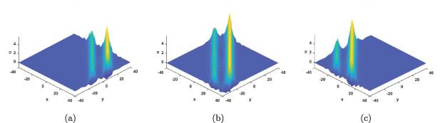
Figure 11. Spatial structure of the breather molecule with $s_1 = s_2 = 1$, $a_1 = 0.2$, $b_1 = 1$, $c_1 = 0.2$, $d_1 = -0.5$, $v_1 = 1$, $w_1 = 0.5$, $\delta_1 = -1$, $\gamma_1 = 0$, $a_3 = 0.2$, $b_3 = 0.8$, $c_3 = 0.2$, $d_3 = -0.5$, $v_3 = -0.135\,834\,8883$, $w_3 = 2$, $\delta_3 = 2$, $\gamma_3 = 0$, $g_1 = t^2$, $g_2 = 2t$. (a) $t = -2$. (b) $t = 0$. (c) $t = 2$. |
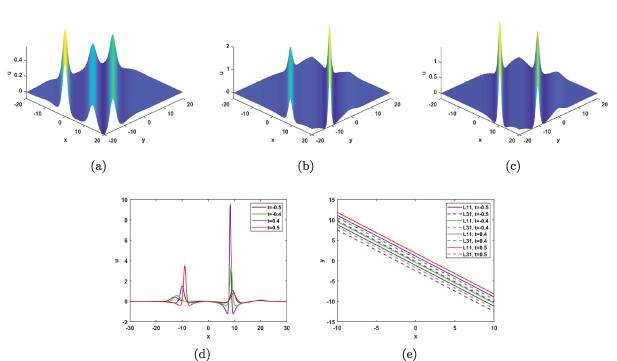
Figure 12. Spatial structure of the transformed wave molecule with $s_1 = s_2 = 1$, $a_1 = 0.3$, $b_1 = 0.4$, $c_1 = 0.3$, $d_1 = 0.4$, $v_1 = 2$, $w_1 = 1$, $\delta_1 = -3$, $\gamma_1 = 0$, $a_3 = 0.4$, $b_3 = 0.2$, $c_3 = 0.4$, $d_3 = 0.2$, $v_3 = 2.403\,037\,858$, $w_3 = 2$, $\delta_3 = -3$, $\gamma_3 = 0$, $g_1 = t^2$, $g_2 = 2t^2$. (a) $t = -1$. (b) $t = 0$. (c) $t = 0.4$. (d) Cross-sectional plots. (e) The characteristic lines solitary wave component. $L_{11}:\ y = -x+ 11.981\,111\,11t^3+0.321$$921\,3960$ and $L_{31}:\ y = -x+ 11.981\,111\,11t^3-0.974\,190\,1390$. |
If conditions (11 ), (13 ) and (20 ) are satisfied, one breather converts into a transformed wave while the other remains unchanged, and thus the specific semi-transition under (13 ) and (20 ) gives rise to a shape-preserving transformed wave-breather molecule as illustrated in figure 13. The dynamical behaviors are shown in figures 13(a)-(c). Unlike the unidirectional propagation in figure 12, figures 13(d) and (e) reveal that this molecular wave exhibits reciprocal propagation, namely, at opposite times ($t$ and $-t$), the wave profiles coincide exactly. This reciprocal behavior stems from the fact that the characteristic lines $L_{11}$ and $L_{31}$ are both even functions of the time variable $t$. Finally, taking two breathers under the complete set of conditions (11 ), (13 ), (19 ), and (20 ) into account, a full-transition and reciprocal shape-preserving transformed wave molecule is constructed and presented in figure 14. Figures 14(a)-(c) exhibit the dynamical evolution of the molecule at $t = \pm1, t = 0$, and $t = \pm2$. Figure 14(d) shows the profiles of the molecule at these different moments. It can be seen that at times $t$ and $-t$, the trajectories coincide completely, indicating that the transformed wave molecule undergoes reciprocal motion while maintaining its shape. This phenomenon is further explained by the coincidence of the characteristic lines at symmetric times and the invariance of their distance shown in figure 14(e). Notably, it is the regulation of the inhomogeneous coefficients in (1 ) that enables this special phenomenon. And thus such dynamics are absent in constant-coefficient systems.
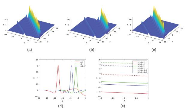
Figure 13. Spatial structure of the transformed wave-breather molecule with $s_1 = s_2 = 1$, $a_1 = b_1 = c_1 = d_1 = 0.4$, $v_1 = 2$, $w_1 = -1.974\,234\,029$, $\delta_1 = 2$, $\gamma_1 = 0$, $a_3 = 0.3$, $b_3 = 1$, $c_3 = 0.3$, $d_3 = -0.5$, $v_3 = 1$, $w_3 = 1.512\,500\,124$, $\delta_3 = -5$, $\gamma_3 = 0$, $g_1 = t$, $g_2 = 2t$. (a) $t = \pm 1$. (b) $t = 0$. (c) $t = \pm0.5$. (d) Cross-sectional plots. (e) The characteristic lines solitary wave component. $L_{11}:\ y = -x - 11.338\,962\,68t^2-4.975$$687\,028 $ and $L_{31}:\ y = -x - 13.071\,652\,52t^2+16.342\,324\,44$. |
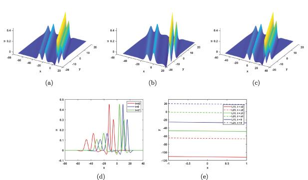


Figure 14. Spatial structure of the transformed wave molecule with $s_1 = s_2 = 1$, $a_1 = b_1 = c_1 = d_1 = 0.3$, $v_1 = 2$, $w_1 = -1.991\,883\,531$, $\delta_1 = 6$, $\gamma_1 = 0$, $a_3 = b_3 = c_3 = d_4 = 0.5$, $v_3 = -3.345\,403\,65$, $w_3 = 3.307\,827\,92$, $\delta_3 = -6$, $\gamma_3 = 0$, $g_1 = t$, $g_2 = 2t$. (a) $t = \pm1$. (b) $t = 0$. (c) $t = \pm2$. (d) Cross-sectional plots. (e) The characteristic lines solitary wave component. $L_{11}:\ y = - x - 21.132\,039\,23t^2-26.646\,333\,98$ and $L_{31}:\ y = - x - 21.132\,039\,16t^2+18.724\,696\,99$. |
7. Conclusion
In this study, the modulation of transformed waves in a $(3+1)$-dimensional variable-coefficient Hirota bilinear system has been systematically investigated. Through characteristic line analysis, we derive the transition condition for breather-to-soliton, and further reveal that a transformed wave arises from the nonlinear superposition of a solitary component and a periodic wave component. The velocity difference between these two components induces a phase difference, which in turn leads to the time-varying property of the transformed wave during propagation. This fundamental property is also valid for constant-coefficient systems, while the introduction of inhomogeneous coefficients in a variable-coefficient system allows for the regulation of phase differences, which make it possible to fix phase differences over time to the same constant. This modulation enables the generation of shape-preserving transformed waves, which is absent in constant-coefficient systems. In addition, by using the characteristic lines technique, parabolic transformed waves, such as quasi-soliton, M-shaped soliton, and multi-peak soliton, are also obtained, whose waveforms can be further tuned through parameter selection.
On the basis of the dynamical behavior of a single wave, many novel interaction solutions are constructed as well. On the one hand, we study the interaction between two transformed waves, namely long-lived collisions and short-lived collisions. In the long-lived collision regime, the characteristic line families of the two breathers remaining intersecting, whereas within the short-lived collision regime, they continually parallel. On the other hand, by utilizing the velocity resonance method, controllable wave molecules of various types are successfully constructed, including breather molecules, transformed wave-breather molecules, and transformed wave molecules. More importantly, the propagation behaviors of the wave molecules can be regulated through the appropriate selection of inhomogeneous coefficients. Specifically, they can be engineered to propagate either unidirectionally or reciprocally, and their waveforms can be controlled to either evolve or remain invariant. These results not only enrich the theory of transformed waves in variable-coefficient systems but also suggest promising applications in controllable wave modulation.
This work deals with the interactions between two waves, but the dynamical mechanisms of multi-wave interactions are considerably more complex and are expected to yield even richer physical phenomena. More interestingly, physical information neural networks could be incorporated into the framework of transformed waves in the high-dimensional variable-coefficient models. These are in progress now and will be reported elsewhere in future.