

1. Introduction
The combination of computer simulations and advanced mathematical sciences is nowadays very essential in applied research. Study like physiological processes offers sophisticated approaches for effectively estimating and predicting complicated outcomes across diverse physiological systems. But because of its complicated activities and detailed structure, understanding the events that take place in the brain is very difficult. Neurons are the basic units or building blocks of the brain. The brain functioning is maintained by the ions concentration like calcium, sodium, potassium etc. in the neurons and its supporting cells. Even a slight modifications or dysfunction lead to generation of tangles and plaques inside and outside the neurons. This may be first sign of the progression of neuronal disorders like Alzheimer's disease (AD). AD symptoms include memory loss, cognitive impairment, and language difficulties [1]. As reported in 2014, over 30 million people around the world have received a diagnosis of AD, one of these neurodegenerative disorders, and this number is predicted to increase soon [2]. Individuals who are above 60 years old are susceptible to such situations. Additionally, compared to adult men, women are more likely to get this ailment. Research indicates that tangles of neurofibrillary cells and amyloid beta plaques are the cause of AD [3]. Plaques form outside of cells, but tangles reside inside them.
Calcium is influenced by several variables, and adjustments to these might alter the regulatory processes [4]. Some of these characteristics have been observed via a few pumps and exchangers, mitochondria, and the endoplasmic reticulum (ER), including voltage-gated calcium channels (VGCC) and the sodium-calcium exchanger (NCX) [2, 4, 5]. Calcium is bound by buffer as it enters the cells, which also lowers the amount of calcium within the cells [3, 6]. The bulk of the calcium is found to be buffered, with only 1% of the calcium (Ca2+) being further sequestered. Any one of these factors dysregulated leads to an increase in intracellular calcium. Bezprozvanny claims that it turns a cell poisonous, interfering with normal physiological processes [7]. The study aims to analyze the impact of ER and buffering agents on calcium diffusion in both healthy cells and affected cells with AD. Buffers, by their interaction with calcium ions, play an important role in controlling intracellular calcium concentrations and hence influencing overall calcium homeostasis [8-11].
In recent years, numerous numerical and analytical approaches have been utilized to explore calcium diffusion levels across different parameters, leading to a deeper insight into intracellular calcium behavior [12-16]. Also, the transport and diffusion of calcium in conjunction using buffers and numerous parameters for regular cells and cells impacted by AD were successfully investigated by researchers [17-18]. A specialized mathematical model has been constructed to deepen our comprehension of calcium signaling in a variety of cell types, including alpha cells, cholangiocytes, oocytes, hepatocytes, and others [19-23]. Maintaining calcium concentration with the help of buffers and the ER can help prevent cell death.
Differential equations play an important role in predicting calcium dynamics in biological systems; nevertheless, their usefulness is frequently restricted by the difficulty of properly specifying initial and boundary conditions, especially in complex brain settings. In actual situations, calcium concentrations are vulnerable to measurement error, biological variability, and experimental noise, rendering standard deterministic models ineffective in capturing true system behavior. To address this limitation, fuzzy differential equations (FDEs) provide a strong mathematical framework for incorporating uncertainty directly into model formulation, allowing for more realistic and informative descriptions of calcium signaling processes and facilitating early detection of neural dysfunctions.
Kaleva contributed to the early development of fuzzy calculus by introducing the Hukuhara derivative, however it was subsequently shown that under this formulation, the uncertainty in solutions might increase unbounded over time [24, 25]. To address this limitation, Bede and colleagues introduced the generalized Hukuhara (gH) derivative and successfully applied it to fuzzy boundary value problems (FBVPs), considerably increasing solution behavior and interpretability [26, 27]. Allahviranloo et al then used a collocation-based strategy to find approximate solutions to nth-order linear differential equations with inaccurate starting and boundary conditions, exhibiting both computing efficiency and accuracy [28, 29]. Gasilov et al made further advances by using linear transformation techniques to solve differential equations with fuzzy boundary values, underlining the advantages of this approach in handling uncertainty effectively [30, 31].
Despite these developments, there have been few research that use FDEs to biologically realistic calcium diffusion models, notably in the setting of neurodegenerative disorders. Existing works using generalized Hukuhara differentiation have shown promise in predicting calcium flow in both healthy and AD-affected cells [32, 33], yet a systematic comparison of solution techniques within this framework remains limited.
Motivated by this gap, the current work uses a FDE model to characterize intracellular calcium diffusion in the presence of buffering mechanisms and ER fluxes. Two unique methodologies are established for addressing the ensuing FBVPs for healthy and AD-affected neurons. A thorough comparative examination of various methodologies is carried out to assess their efficacy, accuracy, and appropriateness for biological interpretation. This comparison not only shows each method's respective merits, but also sheds fresh information on how to use more accurate computational tools for simulating calcium dysregulation in neurodegenerative disorders.
The present model extends classical calcium diffusion frameworks by incorporating fuzzy boundary conditions to capture inherent biological uncertainties, in contrast to traditional deterministic models that assume fixed boundary values. Furthermore, compared to previous models based just on linear diffusion or simpler reaction-diffusion systems, the addition of buffering dynamics and spatial-temporal variations offers a more realistic portrayal. This distinguishes the present method apart from other calcium dynamics models and improves its suitability for intricate intracellular environments. The fuzzy undetermined coefficient approach extends traditional solution techniques to a more realistic environment by providing a structured analytical framework to generate solutions under such uncertainty.
This study primarily focuses on the development and comparative assessment of fuzzy solution methodologies for calcium diffusion models, while parameter settings corresponding to healthy and Alzheimer's-affected cells are analyzed to examine methodological behavior under distinct physiological conditions.
2. Fundamental concepts of fuzzy set theory
Fuzzification is used to incorporate both inherent biological variability and experimental uncertainty in intracellular calcium kinetics. Triangular fuzzy numbers are used for their simplicity and simple biological interpretation in terms of lower, most likely, and upper physiological boundaries. The resulting fuzzy boundary values represent cell-to-cell heterogeneity, stochastic calcium transport, and measurement imprecision, expanding the standard deterministic model.
A fuzzy set $A$ in X is defined by a membership function ${\text{ }}{f_{\text{A}}}\left( x \right)$, which assigns a real number between 0 to 1 to each point in X.
A fuzzy interval is defined as ${\text{ }}{\underline {L}} < \bar L$, while a fuzzy number is defined as ${\text{ }}{\underline {L}} = \bar L$. As a conventional form, the imprecise number will be regarded as superior semi-continuous with support interval $\left[ {\underline {{L_0}} ,\overline {{L_0}} {\text{ }}} \right]$ of w, which is also closed and restricted.
| • | ($\text { ● }$)$ \alpha - {\text{cuts}}$ of ${\text{ }}L$ is denoted by ${\text{ }}{{{L}}_ \alpha }$, where $ \alpha $ is an integer between 0 and 1, and the lower and higher branches of ${\text{ }}L$ are denoted by ${\underline {L}} $, $\bar L$ respectively. |
| • | ($\text { ● }$)$w = \langle p,r,q\rangle $ represents the triangular-shaped fuzzy membership value and $ \alpha - {\text{cut}}$ is noted as $\begin{equation*}{\left[ L \right]^ \alpha } = \left[ {\underline {{L_ \alpha }} ,\overline {{L_ \alpha }} {\text{ }}} \right] = \left[ {p + \left( {r - p} \right) \alpha ,{\text{ }}q + \left( {r - q} \right) \alpha } \right].\end{equation*}$ |
Assuming a triangular fuzzy number $\tilde L = \left\langle {a,0,b} \right\rangle $ with 0 as a vertex. So, we can state that ${\underline {L}} = \left( {1 - \alpha } \right)a$ and ${\text{ }}\bar L = \left( {1 - \alpha } \right)b$. If we examine ${\text{ }}0 - \text{cut}$, with interval ${\text{ }}\left[ {a,b} \right]$, and coefficient ${\text{ }}\left( {1 - \alpha } \right)$. $\tilde L = {L_{\text{cr}}} + {\tilde L_{\text{un}}}$ is a way to express the fuzzy number $\tilde w$ where ${L_{\text{cr}}}$ the crisp portion with a unit degree of membership and ${\tilde L_{\text{un}}}$ is considered as an imprecise element with its midpoint acting as an edge.
In this study, Hukuhara differentiability has been considered. The concept of differentiability according to Hukuhara (H-derivative) for fuzzy function relies on the H-difference of sets.
At the point ${\text{ }}{h_0}:\left( {a,b} \right) \to {{\mathbb{R}}_\mathcal{F}}$, the strong gH-differentiability of a fuzzy-valued function is characterized as:
Considering $k^{\prime}\left( {{h_0}} \right) \in {{\mathbb{R}}_\mathcal{F}}$ for all $z > 0$ adequately tiny, $\exists k\left( {{h_0} + z} \right)\circleddash k\left( {{h_0}} \right),$ again there exists $k\left( {{h_0}} \right)\circleddash k\left( {{h_0} - z} \right)$ and the limit is maintained as
$\begin{align*}k^{\prime}\left( {{h_0}} \right) = \mathop {\lim }\limits_{z \to 0} \frac{{k\left( {{h_0} + z} \right)\circleddash k\left( {{h_0}} \right)}}{{z{\text{ }}}} = \mathop {\lim }\limits_{z \to 0} \frac{{k\left( {{h_0}} \right)\circleddash k\left( {{h_0} - z} \right)}}{{z{\text{ }}}},\end{align*}$
where ${{\mathbb{R}}_\mathcal{F}}$ is a collection of all fuzzy numbers. The following is an expression for the approximate solution obtained by applying the undetermined fuzzy coefficients method [28]: $\begin{align*}{\tilde Z_\beta }\left( x \right) = \mathop \sum \limits_{\gamma = 0}^\beta {\tilde \theta _\gamma }{\varphi _\gamma }\left( x \right).\end{align*}$
where ${\text{ }}{\varphi _\gamma }\left( x \right),{\text{ }}\gamma = 0,1,2, \ldots , \beta $, are positive differentials and are positive functions.Lemma 1 [28]: Assume that all positive differential equations have a positive value for the fundamental function ${\varphi _\gamma }\left( x \right),{\text{ }}\gamma = 0,1,2, \ldots ,\beta $, then ${\left( {\underline {{Z_\beta }} } \right)^j}\left( x \right) = \underline {{Z_\beta }^j} \left( x \right)$ and ${\text{ }}{\left( {\overline {{Z_\beta }} } \right)^j}\left( x \right) = \overline {{Z_\beta }^j} \left( x \right)$, $j = 0,1,2$.
3. The approaches for solving the boundary value problem with fuzzy conditions
3.1. Undetermined fuzzy coefficient approach
The 2nd order differential equation with linear form can be expressed as
$\begin{align}z^{^{\prime}\! ^{\prime} } = f\left( {v,x,x^{\prime}} \right),\quad \boldsymbol{v} \in \left[ {a,b} \right].\end{align}$
With condition
$\begin{align}x\left( a \right) = {\tilde k_1},\quad x\left( b \right) = {\tilde k_2},\quad {\tilde k_1},{\tilde k_2} \in {\mathbb{R}_\mathcal{F}}.\end{align}$
The suggested method can be stated as [39]
$\begin{align}{\tilde X_\beta }\left( v \right) = \mathop \sum \limits_{\gamma = 0}^\beta {\tilde \theta _\gamma }{\varphi _\gamma }\left( \boldsymbol{v} \right).\end{align}$
After putting equations (1 ) and (2 ) in equation (3 ) the parametric forms can be written as
$\begin{align}\left\{ {\begin{array}{*{20}{l}} {\underline {x^{^{\prime}\! ^{\prime} }} \left( {{\boldsymbol{v}}, \alpha } \right) + s\left( {\boldsymbol{v}} \right)\underline {x^{\prime}} \left( {{\boldsymbol{v}}, \alpha } \right) + t\left( {\boldsymbol{v}} \right){\underline {x}} \left( {{\boldsymbol{v}}, \alpha } \right) = {\underline {w}} \left( {{\boldsymbol{v}}, \alpha } \right),} \\ {{\underline {x}} \left( {a, \alpha } \right) = \underline {{k_1}} \left( \alpha \right),} \\ {{\underline {x}} \left( {b, \alpha } \right) = \underline {{k_2}} \left( \alpha \right),} \\ {\overline {x^{^{\prime}\! ^{\prime} }} \left( {{\boldsymbol{v}}, \alpha } \right) + s\left( {\boldsymbol{v}} \right)\overline {x^{\prime}} \left( {{\boldsymbol{v}}, \alpha } \right) + t\left( {\boldsymbol{v}} \right)\bar x\left( {{\boldsymbol{v}}, \alpha } \right) = \bar w\left( {{\boldsymbol{v}}, \alpha } \right),} \\ {\bar x\left( {a, \alpha } \right) = \overline {{k_1}} \left( \alpha \right),} \\ {\bar x\left( {b, \alpha } \right) = \overline {{k_2}} \left( \alpha \right).} \end{array}} \right.\end{align}$
To find the solution of equation (4 ) with $s\left( v \right)$ is negative and $t\left( v \right)$ is non negative, the system has been obtained as follows:
$\begin{equation}\left\{ \begin{array}{*{20}{l}} \mathop \sum \limits_{\gamma = 0}^\beta \underline {{\theta _\gamma }} \left( \alpha \right){\delta _\gamma } + \mathop \sum \limits_{\gamma = 0}^\beta \overline {{\theta _\gamma }} \left( \alpha \right){\chi _\gamma } = \underline {w}\left( {{\boldsymbol{v}}, \alpha } \right), \\ \mathop \sum \limits_{\gamma = 0}^\beta \underline {{\theta _\gamma }} \left( \alpha \right){\sigma _{a\gamma }} = \underline {{k_1}} \left( \alpha \right), \\ \mathop \sum \limits_{\gamma = 0}^\beta \underline {{\theta _\gamma }} \left( \alpha \right){\sigma _{b\gamma }} = \underline {{k_2}} \left( \alpha \right), \\ \mathop \sum \limits_{\gamma = 0}^\beta \overline {{\theta _\gamma }} \left( \alpha \right){\delta _\gamma } + \mathop \sum \limits_{\gamma = 0}^\beta \underline {{\theta _\gamma }} \left( \alpha \right){\chi _\gamma } = \bar w\left( {{\boldsymbol{v}}, \alpha } \right), \\ \mathop \sum \limits_{\gamma = 0}^\beta \overline {{\theta _\gamma }} \left( \alpha \right){\sigma _{a\gamma }} = \overline {{k_1}} \left( \alpha \right), \\ \mathop \sum \limits_{\gamma = 0}^\beta \overline {{\theta _\gamma }} \left( \alpha \right){\sigma _{b\gamma }} = \overline {{k_2}} \left( \alpha \right), \end{array} \right.\end{equation}$
where the notations can be expressed as $\begin{align*}&{\delta _\gamma } = \varphi _\gamma ^{^{\prime}\! ^{\prime} }\left( {\boldsymbol{v}} \right) + s\left( {\boldsymbol{v}} \right)\varphi _\gamma ^{\prime}\left( {\boldsymbol{v}} \right),{\chi _\gamma } = - t\left( {\boldsymbol{v}} \right){\varphi _\gamma }\left( {\boldsymbol{v}} \right),{\sigma _{a\gamma }} = {\varphi _\gamma }\left( a \right),\nonumber\\ & {\sigma _{b\gamma }} = {\varphi _\gamma }\left( b \right),\gamma = 0,1,2, \ldots ,\beta .\end{align*}$
From the above, system (5 ) exists in the form $\boldsymbol{{S}}\left( v \right)\boldsymbol{{x}}\left( \alpha \right) = \boldsymbol{z}\left( \alpha \right)$
$\begin{align*}\boldsymbol{S} &= \left[ {\begin{array}{*{20}{c}} {{\boldsymbol{S}_1}}&{{\boldsymbol{S}_2}} \\ {{\boldsymbol{S}2}}&{{\boldsymbol{S}_1}} \end{array}} \right]{\text{and}}\,\,\,{\boldsymbol{S}_1} = \left[ {\begin{array}{*{20}{c}} {{\delta _0}}&{{\delta _1}} & \cdots & {{\delta _\beta }} \\ {{\sigma _{a0}}} &{{\sigma _{a1}}} &\cdots &{{\sigma _{a\beta }}}\\ {{\sigma _{b0}}}& {{\sigma _{b1}}} &\cdots&{{\sigma _{b\beta }}}\end{array}} \right],\nonumber\\ {\boldsymbol{S}_2} &= \left[ {\begin{array}{*{20}{c}} {{\chi _0}}&{{\chi _1}}&{\begin{array}{*{20}{c}} \cdots &{{\chi _\beta }} \end{array}} \\ 0&0&{\begin{array}{*{20}{c}} \cdots &0 \end{array}} \\ 0&0&{\begin{array}{*{20}{c}} \cdots &0 \end{array}} \end{array}} \right].\end{align*}$
Moreover, ${\text{ }}\boldsymbol{x} = {\left( {\underline {{\theta _0}} ,{\text{ }}\underline {{\theta _1},} \ldots ,\underline {{\theta _\beta }} ,\overline {{\theta _0}} ,\overline {{\theta _1}} , \ldots ,\overline {{\theta _\beta }} } \right)^{\text{T}}}.$
$\begin{equation*}\boldsymbol{z} = {\left( {{\underline {w}} \left( {{\boldsymbol{v}}, \alpha } \right),{\text{ }}\underline {{k_1}} \left( \alpha \right),\underline {{k_2}} \left( \alpha \right),\bar w\left( {{\boldsymbol{v}}, \alpha } \right),\overline {{k_1}} \left( \alpha \right),\overline {{k_2}} \left( \alpha \right)} \right)^{\text{T}}}.\end{equation*}$
By solving (5 ) with taking ${\text{ }}\boldsymbol{v} = d,{\text{ }}d \in \left[ {a,b} \right]$, considering the aforementioned $\underline {{\theta _0}} ,{\text{ }}\underline {{\theta _1},} \ldots ,\underline {{\theta _\beta }} ,{\text{ }}\overline {{\theta _0}} ,\overline {{\theta _1}} , \ldots ,\overline {{\theta _\beta }} $ can be found. Following that an approximate solution ${\text{ }}\left( {{\underline {x}} \left( {v, \alpha } \right),\bar x\left( {v, \alpha } \right)} \right)$ can be derived.
Thus, the following represents an approximate solution
$\begin{align}\left\{ {\begin{array}{*{20}{c}} {{\underline {x}} \left( {{\boldsymbol{v}}, \alpha } \right) = \underline {{\theta _0}} \left( \alpha \right){\varphi _0}\left( {\boldsymbol{v}} \right) + \underline {{\theta _1}} \left( \alpha \right){\varphi _1}\left( {\boldsymbol{v}} \right) + \ldots + \underline {{\theta _\beta }} \left( \alpha \right){\varphi _\beta }\left( {\boldsymbol{v}} \right),} \\ {\bar x\left( {{\boldsymbol{v}}, \alpha } \right) = \overline {{\theta _0}} \left( \alpha \right){\varphi _0}\left( {\boldsymbol{v}} \right) + \overline {{\theta _1}} \left( \alpha \right){\varphi _1}\left( {\boldsymbol{v}} \right) + \ldots + \overline {{\theta _\beta }} \left( \alpha \right){\varphi _\beta }\left( {\boldsymbol{v}} \right).} \end{array}} \right.\end{align}$
3.2. Analytical approach using linear transformation
Assuming the 2nd order linear differential equation (1 ) with the fuzzy boundary conditions (2 ) can be written as follows
$\begin{align} & z^{^{\prime}\! ^{\prime} } + {a_1}\left( {\boldsymbol{v}} \right)z^{\prime} + {a_2}\left( {\boldsymbol{v}} \right)z = g\left( {\boldsymbol{v}} \right), \nonumber\\ & z\left( a \right) = {{\tilde k}_1}, \nonumber\\ & z\left( b \right) = {{\tilde k}_2}, \end{align}$
where ${\tilde k_1}$ and ${\tilde k_2}$ are fuzzy numbers, while ${a_1}$, ${a_2}$, and $g\left( v \right)$ are crisp functions or constants. Muzzioli and Reynaerts portray fuzzy boundary values as both the crisp and uncertain parts [40], $\begin{align*}{\tilde k_1} = {a_{\text{cr}}} + \tilde a\,\,\,{\text{and}}\,\,\,{\tilde k_2} = {b_{\text{cr}}} + \tilde b.\end{align*}$
The linearity of the differential operator justifies this decomposition. The solution can be written as the sum of a crisp component and an uncertain component since the governing equation is linear and the principle of superposition is applicable. The original FBVP can be equivalently divided into a homogeneous problem with fuzzy boundary conditions and a non-homogeneous crisp problem by expressing the fuzzy boundary values as the sum of their crisp and uncertain components.
The FBVP (7 ) is now divided into the following two sections:
| • | ($\text { ● }$)Non-homogeneous crisp problem: $\begin{align} & z^{^{\prime}\! ^{\prime} } + {a_1}\left( {\boldsymbol{v}} \right)z^{\prime} + {a_2}\left( {\boldsymbol{v}} \right)z = g\left( {\boldsymbol{v}} \right), \nonumber\\ & z\left( a \right) = {a_{\text{cr}}}, \nonumber\\ & z\left( b \right) = {b_{\text{cr}}},\end{align}$ |
| • | ($\text { ● }$)Homogeneous fuzzy problem: $\begin{align} & z^{^{\prime}\! ^{\prime} } + {a_1}\left( {\boldsymbol{v}} \right)z^{\prime} + {a_2}\left( {\boldsymbol{v}} \right)z = g\left( {\boldsymbol{v}} \right), \nonumber\\ & z\left( a \right) = \tilde a, \nonumber\\ & z\left( b \right) = \tilde b .\end{align}$ |
If the solutions of (8 ) and (9 ) are ${z_{\text{cr}}}\left( v \right)$ and ${\tilde z_{\text{un}}}\left( v \right)$ respectively, consequently the solution of (7 ) can be expressed as
$\begin{align}\tilde Z = {z_{\text{cr}}} + {\tilde z_{\text{un}}}.\end{align}$
The crisp solution is unique [41] and can be found in any analytical and numerical approach. There are several ways to interpret the solution of fuzzy equations. The following membership function, as stated by [40, 41] establishes ${\tilde W}$ as the solution to the problem
$\begin{align}{\mu _{\tilde z}}\left( z \right) = \left\{ {\begin{array}{*{20}{c}} {\text{min}\left\{ {{\mu _{\tilde a^{\prime}}}\left( {z\left( \gamma \right)} \right),{\mu _{\tilde b^{\prime}}}\left( {z\left( \beta \right)} \right)} \right\},}&{\text{if }\,z^{^{\prime}\! ^{\prime} } + {b_1}\left( x \right)z^{\prime} + {b_2}\left( x \right)z = 0} \\ 0&{\text{otherwise}} \end{array}} \right.\end{align}$
Let us assume, ${z_1}\left( {\boldsymbol{v}} \right)$ and ${z_2}\left( {\boldsymbol{v}} \right)$ are the distinct solutions of the homogeneous equation. Also, assume that $\boldsymbol{S}\left( {\boldsymbol{v}} \right) = \left( {{z_1}\left( {\boldsymbol{v}} \right),{\text{ }}{z_2}\left( {\boldsymbol{v}} \right)} \right)$, and $\mathbb{u} = \left( {a,b} \right)$.
So, we have
$\begin{align}Z\left( {\boldsymbol{v}} \right) = \boldsymbol{S}\left( {\boldsymbol{v}} \right){\boldsymbol{M}^{ - 1}},\end{align}$
where $\boldsymbol{M} = \left[ {\begin{array}{*{20}{c}} {{z_1}\left( a \right)}&{{z_2}\left( a \right)} \\ {{z_1}\left( b \right)}&{{z_2}\left( b \right)} \end{array}} \right]$ is non-singular matrix and $\left( {{z_1}\left( {\boldsymbol{v}} \right),{\text{ }}{z_2}\left( {\boldsymbol{v}} \right)} \right) = \left( {{z_1}\left( {\boldsymbol{v}} \right),{\text{ }}{z_2}\left( {\boldsymbol{v}} \right)} \right).{\boldsymbol{M}^{ - 1}}$, then the unique solution is [31, 42].$\begin{align*}{\tilde {\text{Z}}}\left( {\boldsymbol{v}} \right) = {z_1}\left( {\boldsymbol{v}} \right){\tilde {\text{a}}} + {z_2}\left( {\boldsymbol{v}} \right){\tilde b}.\end{align*}$
Finally, the solution of (7 ) can be represented as
$\begin{align}\tilde Z\left( {\boldsymbol{v}} \right) = {z_{\text{cr}}}\left( {\boldsymbol{v}} \right) + {z_1}\left( {\boldsymbol{v}} \right)\tilde a + {z_2}\left( {\boldsymbol{v}} \right)\tilde b.\end{align}$
3.3. When using a fuzzy triangular number to indicate boundary values
${\tilde k_1}$ and ${\tilde k_2}$ are two boundary conditions which is a triangular fuzzy numbers. They represent equal intervals that are inserted to form a triangular fuzzy number ${\tilde Z}\left( {v} \right)$. The representation of it is $\tilde Z\left( {\boldsymbol{v}} \right) = \left( {\underline {{z_0}} \left( {\boldsymbol{v}} \right),0,\overline {{z_0}} \left( {\boldsymbol{v}} \right)} \right)$. Let us assume that ${\tilde k_1} = \left( {\underline {{a_0}} ,0,\overline {{a_0}} } \right){\text{and}}\,{\tilde k_2} = \left( {\underline {{b_0}} ,0,\overline {{b_0}} } \right)$. Also, assume that $z\left( {\boldsymbol{v}} \right) = (\left( {{z_1}\left( {\boldsymbol{v}} \right),{z_2}\left( {\boldsymbol{v}} \right)} \right)$ then the maximum and minimum values throughout the products can be written as
$\begin{align*}z\left( x \right) \cdot {\mathbb{u}} = {k_1}{z_1}\left( x \right) + {k_2}{z_2}\left( x \right).\end{align*}$
4. Mathematical framework
Mathematical modeling of the systems governing these physiological processes aids in identifying the key factors influencing them and enables computational analysis. This section outlines the mathematical framework of the caleium buffering dynamics. A two-dimensional partial differential equation has been formed, incorporating the effects of buffer and ER, to highlight the role of these parameters in neuronal disorders like AD.
4.1. Calcium buffering
Calcium ions diffuse into the cytosol and bind with buffers (proteins), resulting in the formation of calcium-bound buffers. Studies have revealed that there is a considerable decrease in buffer proteins in AD, which subsequently causes an increase in intracellular calcium levels [6]. The buffers at the cytosol's periphery are interacting with unbound calcium ions in the brain. The following is the mathematical expression for a physiological process known as calcium buffering [6, 43].
$\begin{equation}\left[ {\text{C}{\text{a}^{2 + }}} \right] + {\text{ }}\left[ B \right] = {\text{ }}\left[ {\text{Ca}B{\text{ }}} \right],\end{equation}$
where [${\text{Ca}B}$] and [${{B}}$] are bound and unbound buffers respectively. The partial differential equations that are produced, which are based on Fickian diffusion, have the following form [44, 45]: $\begin{align}\frac{{\partial C}}{{\partial t}} &= {D_{{\text{Ca}}}}\left( {\frac{{{\partial ^2}C}}{{\partial {x^2}}} + \frac{{{\partial ^2}C}}{{\partial {y^2}}}} \right) + \sum\limits_j {R_j} + {\sigma _{{\text{Ca}}}},\end{align}$
$\begin{align}\frac{{\partial \left[ {{B}} \right]}}{{\partial t}} &= {D_{{{{B}}_j}}}\left( {\frac{{{\partial ^2}\left[ {{B}} \right]}}{{\partial {x^2}}} + \frac{{{\partial ^2}\left[ {{B}} \right]}}{{\partial {y^2}}}} \right) + {R_j},\end{align}$
$\begin{align}\frac{{\partial \left[ {{\text{Ca}B}} \right]}}{{\partial t}}& = {D_{{\text{Ca}B}}}\left( {\frac{{{\partial ^2}\left[ {{\text{Ca}B}} \right]}}{{\partial {x^2}}} + \frac{{{\partial ^2}\left[ {{\text{Ca}B}} \right]}}{{\partial {y^2}}}} \right) - {R_j},\end{align}$
where, $\begin{align}{R_j} = - {k_j}^ + \left[ {{B}} \right]\left[ {{\text{Ca}}} \right] + {k_j}^ - \left[ {{\text{Ca}B}} \right].\end{align}$
Here, ${\text{ }}{{{D}}_{{\text{Ca}}}}$ refers to the diffusion parameter of unbound calcium ions, while ${{{D}}_{{{{B}}_{\text{j}}}}}{\text{ as well as }}{{{D}}_{{\text{Ca}B}}}$ denote the diffusion coefficients for buffers that bind calcium and calcium that are bound to calcium respectively. Furthermore, the rate of association and dissociation for the buffer are indicated by ${\text{ }}{{{k}}_{\text{j}}}^ + {\text{ }}and{\text{ }}{{{k}}_{\text{j}}}^ - {\text{ }}$.
4.2. Endoplasmic Reticulum
It is theoretically assumed that through that the commencement of calcium flow from the ER, the total concentration of calcium ions within a cell would remain constant, and calcium exchange with mitochondria and calcium absorption does not need to be taken into consideration [46]. The ${\text{C}}{{\text{a}}^{2 + }}$ conservation can be expressed as [45],
$\begin{align}{C_1} = \frac{{{V_{{\text{ER}}}}}}{{{V_{{\text{Cyt}}}}}},{C_0} = {C_1}{\left[ {{\text{C}}{{\text{a}}^{2 + }}} \right]_{{\text{ER}}}} + {\left[ {{\text{C}}{{\text{a}}^{2 + }}} \right]_i},\end{align}$
where, ${\left[ {{\text{C}}{{\text{a}}^{2 + }}} \right]_{{\text{ER}}}} = \frac{{{\eta _{{\text{ER}}}}}}{{{V_{{\text{ER}}}}}}\,\,\,{\text{and}}\,\,\,{\left[ {{\text{C}}{{\text{a}}^{2 + }}} \right]_i} = \frac{{{\eta _{{\text{Cyt}}}}}}{{{V_{{\text{Cyt}}}}}}.$Here, ${\text{ }}{{\text{C}}_0}{\text{ represents the overall calcium concentration}}$ and ${\text{ }}{C_1}$ represents the ER to Cytosol volume ratio.
We have
$\begin{align}\frac{{{\text{d}}{{\left[ {{\text{C}}{{\text{a}}^{2 + }}} \right]}_i}}}{{{\text{d}}t}} = {C_1}\left[ {{J_{{\text{leak}}}} + {J_{{\text{chan}}}}} \right] - {J_{{\text{pump}}}}.\end{align}$
The outward fluxes through ${J_{{\text{leak}}}}$ and ${\text{ }}{J_{{\text{chan}}}}$ are computed using Fick's law and are provided below [45]
$\begin{align}{J_{{\text{leak}}}} = \frac{{{D_{{\text{leak}}}}}}{{{C_1}}}\left( {1 + {C_1}} \right)\left( {\frac{{{C_0}}}{{1 + {C_1}}} - {{\left[ {{\text{C}}{{\text{a}}^{2 + }}} \right]}_i}} \right),\end{align}$
$\begin{align}{J_{\text{chan}}} = \frac{{{D_{\text{chan}}}}}{{{C_{{\text{ }}1}}}}\left( {1 + {C_1}} \right)\left( {\frac{{{C_0}}}{{1 + {C_1}}} - {{\left[ {C{a^{2 + }}} \right]}_i}} \right),\end{align}$
where ${\text{ }}{{{D}}_{{\text{leak}}}}{\text{ and}}$ ${D_{{\text{chan}}}}$ are considered as diffusivity constant and channel conductivity.Furthermore as seen below, the inward flow ${J_{{\text{pump}}}}$ is obtained by applying the Michaelis-Menten equation with a Hill coefficient set to 2
$\begin{align}{J_{{\text{pump}}}} = P_{{\text{max}}}^{\text{R}}\frac{{{{\left[ {{\text{C}}{{\text{a}}^{2 + }}} \right]}_i}^2}}{{{{\left[ {{\text{C}}{{\text{a}}^{2 + }}} \right]}_i}^2 + {{\left[ {K_{\text{R}}^{\text{M}}} \right]}^2}}},\end{align}$
where ${{ P}}_{{\text{max }}}^{\text{R}}{\text{and }} K_{\text{R}}^{\text{M}}$ represents a maximum pump rate and Michaelis-Menten constantThe parameter values were chosen from physiologically described ranges in the literature and are in line with calcium dynamics that have been seen experimentally in both normal and diseased circumstances. All the factors used to find the solution are taken from table 1.
Table 1. Notation table. |
| Symbol | Description |
|---|---|
| $z\left( {\boldsymbol{v}} \right)$ | Unknown variable of the function $v$ |
| $v$ | Independent variable |
| ${a_1}\left( {\boldsymbol{v}} \right),{a_2}\left( {\boldsymbol{v}} \right)$ | Coefficient functions |
| $g\left( v \right)$ | Nonhomogeneous term |
| ${\tilde k_1}$, ${\tilde k_2}$ | Fuzzy boundary values at $v = a$ and $v = b$ |
| ${\varphi _\gamma }\left( x \right)$ | Positive differentials and positive functions |
| ${{\mathbb{R}}_\mathcal{F}}$ | Collection of fuzzy numbers |
| $ \alpha - {\text{cut}}$ | A crisp set of elements whose membership in a fuzzy set is greater than or equal to a given threshold a |
5. Statement of the problem
The ER, calcium-binding buffers, and a two-dimensional partial differential equation are taken into consideration in the following model
$\begin{align}& {D_x}\frac{{{\partial ^2}C}}{{\partial {x^2}}} + {D_y}\frac{{{\partial ^2}C}}{{\partial {y^2}}} + \left( {1 + {C_1}} \right)\left( {{D_{\text{leak}}} + {D_{\text{chan}}}} \right) \times \left( {\frac{{{C_0}}}{{1 + {C_1}}} - C} \right)\nonumber\\ &\quad - P_{\text{max}}^{\text{R}}\left( {\frac{{{C^2}}}{{{C^2} + {K^2}}}} \right) - {k^ + }{B_\infty }{\text{ }}\left[ {C - {C_\infty }} \right] = 0.\end{align}$
Considering, a new space variable as [47]
$\begin{equation}X = x + y\sqrt {\frac{{{D_y}}}{{{D_x}}}} .\end{equation}$
Assuming that the calcium concentration varies primarily along the direction defined by ${\text{ }}X$,
$\begin{align*}C\left( {x,y} \right) = C\left( X \right).\end{align*}$
The second order spatial derivatives transform as
$\begin{align*}\frac{{{\partial ^2}C}}{{\partial {x^2}}} + \frac{{{D_y}}}{{{D_x}}}\frac{{{\partial ^2}C}}{{\partial {{\text{y}}^2}}} = \frac{{{{\text{d}}^2}C}}{{{\text{d}}{X^2}}}.\end{align*}$
Dividing (24 ) by ${D_x}$ and applying the above transformation yields an effective one-dimensional ordinary differential equation.
Therefore, the equation (24 ) can be written as follows:
$\begin{align}\frac{{{{\text{d}}^2}C}}{{{\text{d}}{X^2}}} - pC + q = 0.\end{align}$
The model, which is a computationally efficient approximation that incorporates the key aspects of intracellular calcium transport, is developed in two spatial dimensions. The 2D assumption is suitable for assessing spatial changes in calcium because neural structures can be locally modeled as planar domains at the subcellular scale. While simplifying the above equation, the term that is non-linear can be addressed in the following approaches:
5.1. Case-I
For $C \ll {{K}}$, $\frac{{{C^2}}}{{{C^2} + {K^2}}} < \frac{{{C^2}}}{{{K^2}}} < \frac{C}{K},$
$\begin{align}\frac{{{{\text{d}}^2}C}}{{{\text{d}}{X^2}}} - {p_1}C + {q_1} = 0,\end{align}$
where, $\begin{align} & {p_1} = \frac{1}{D}\left[ {\left( {1 + {c_1}} \right)\left( {{D_{{\text{leak}}}} + {D_{{\text{chan}}}}} \right) + \frac{{P_{\text{R}}^{{\text{max}}}}}{K} + {k^ + }{B_\infty }} \right],\end{align}$
$\begin{align} & {q_1} = \frac{1}{D}\left[ {{c_0}\left( {{D_{{\text{leak}}}} + {D_{{\text{chan}}}}} \right) + {k^ + }{B_\infty }{c_\infty }} \right].\end{align}$
5.2. Case-II
For ${\text{ }}C \gg {{K}}$, ${{ K}} = {{\gamma }}C{\text{ }}$, $0 < \gamma < 1$
$\begin{align}\frac{{{{\text{d}}^2}C}}{{{\text{d}}{X^2}}} - {p_2}C + {q_2} = 0,\end{align}$
where, $\begin{align*} & {p_2} = \frac{1}{D}\left[ {\left( {1 + {c_1}} \right)\left( {{D_{{\text{leak}}}} + {D_{{\text{chan}}}}} \right) + {k^ + }{B_\infty }} \right],\\ & {q_2}= \frac{1}{D}\left[ {{c_0}\left( {{D_{{\text{leak}}}} + {D_{{\text{chan}}}}} \right) + \frac{{P_{\text{R}}^{{\text{max}}}}}{{{\delta ^2} + 1}} + {k^ + }{B_\infty }{c_\infty }} \right].\end{align*}$
Equations are stated in nondimensional form after scaling the governing variables with suitable characteristic length, time, and concentration scales. The parameters selected from the literature (table 2) are normalized appropriately, maintaining dimensional consistency across diffusion, reaction, and flux terms. To maintain the balance of calcium profile in neuron cells, proper functioning of these factors is very crucial. The boundary conditions which are used as follows:
$\begin{align*}c &= 0,\quad{\text{x}} \unicode{x2A7E} 0,{\text{ y}} \unicode{x2A7E} 0.\end{align*}$
$\begin{align*}c &= {c_0},\quad x = 0, y = 0.\end{align*}$
Table 2. Different parameter values. |
| Expression | Factor | Values | Units | References |
|---|---|---|---|---|
| ${k_j}^ + $ | Association rate | 120 | $\mu {{\text{M}}^{ - 1}}/{\text{s}}$ | [6] |
| ${{B}}$ | Overall buffer concentration | 50-300 | ${{\mu }}{{\text{M}}^{ - 1}}/{\text{s}}$ | [6] |
| ${\left[ {{\text{C}}{{\text{a}}^{2 + }}} \right]_\infty }$ | Background concentration of calcium | 0.1 | $\mu {\text{M}}$ | [6] |
| K | Calcium dissociation constant to pump | 0.1 | $\mu {\text{M}}$ | [6] |
| ${D_{{\text{chan}}}}$ | Capacitance of channel | 6 | ${{\text{s}}^{ - 1}}$ | [44] |
| ${D_{{\text{leak}}}}$ | Leak flux constant of calcium | 0.11 | ${{\text{s}}^{ - 1}}$ | [44] |
| $P_{\text{R}}^{{\text{max}}}$ | Optimal calcium absorption | 0.9 | ${{\mu M}}/{\text{s}}$ | [44] |
| ${C_0}$ | Total calcium concentration | 1 | $\mu {\text{M}}$ | [6] |
| ${C_1}$ | The ER to cytosol volume ratio | 0.185 | - | [6] |
| ${D_{{\text{ca}}}}$ | Diffusion coefficient | 300 | ${{\mu }}{{\text{M}}^2}/{\text{s}}$ | [44] |
This work uses fuzzy logic to describe calcium concentration dynamics due to the inherent imprecision and uncertainty in biological systems, particularly at the cellular level. Unlike deterministic models, which require precise input values, and stochastic models, which rely on probabilistic distributions, fuzzy logic enables the direct representation of ambiguous or imprecise biological information, such as varying boundary concentrations caused by cellular heterogeneity, experimental limitations, or measurement noise. This makes fuzzy modeling ideal for portraying the slow shifts and unpredictability in calcium transmission that occur in complicated biological contexts.
The boundary conditions are represented as fuzzy values to account for inherent biological variability and inadequate physiological knowledge of calcium fluxes across cellular and ER membranes. This technique allows for a more accurate and robust portrayal of intracellular calcium dynamics in healthy and AD-affected cells. The following is an explanation of the way boundary conditions are represented in relation to triangular fuzzy numbers.
$\begin{equation*}\tilde C\left( 0 \right) = \left[ {2 + \alpha ,3.5 - 0.5 \alpha } \right],\,\,\,\tilde C\left( 1 \right) = \left[ { \alpha ,1.5 - 0.5 \alpha } \right].\end{equation*}$
The triangular fuzzy boundary values are presented as phenomenological representations of uncertainty, rather than scientifically calibrated values. Because there is a dearth of exact physiological knowledge on calcium fluxes at cellular and ER membranes, particularly under pathological situations, the boundary values are chosen to keep within physiologically plausible concentration values while also allowing for model sensitivity analysis. The goal of these fuzzy intervals is to investigate the effect of bounded uncertainty on calcium dynamics, not to replicate specific experimental results.
6. Solution of linear FBVP
6.1. Solution by undetermined fuzzy coefficient
There are no significant differences among the cases mentioned above. Therefore to demonstrate solution, consider only case-1. To solve the above problem (27 ), let us assume ${\text{ }}{\emptyset _{{n}}}\left( x \right) = {{{x}}^{{n}}}$, ${\text{ }}n = 0,1,2$. So, the solution for the above problem in upper and lower cases can be represented as follows:
$\begin{align}{\underline {C}} \left( {x, \alpha } \right) = \underline {{\beta _0}} + \underline {{\beta _1}} x + \underline {{\beta _2}} {x^2},\,\,\,{\text{ }}\bar C\left( {x, \alpha } \right) = \overline {{\beta _0}} + \overline {{\beta _1}} x + \overline {{\beta _2}} {x^2}.\end{align}$
Satisfying the above to differential equation (27 ) and given boundary conditions, the following system is obtained,
$\begin{align}&\left[ {\begin{array}{*{20}{c}} 0&0&2&{ - {p_1}}&{ - {p_1}x}&{ - {p_1}{x^2}} \\ 1&0&0&0&0&0 \\ 1&1&1&0&0&0 \\ { - {p_1}}&{ - {p_1}x}&{ - {p_1}{x^2}}&0&0&2 \\ 0&0&0&1&0&0 \\ 0&0&0&1&1&1 \end{array}} \right]\left[ {\begin{array}{*{20}{c}} {\underline {{\beta _0}} } \\ {\underline {{\beta _1}} } \\ {\underline {{\beta _2}} } \\ {\overline {{\beta _0}} } \\ {\overline {{\beta _1}} } \\ {\overline {{\beta _2}} } \end{array}} \right]= \left[ {\begin{array}{*{20}{c}} { - {q_1}} \\ {2 + \alpha } \\ \alpha \\ { - {q_1}} \\ {3.5 - 0.5 \alpha } \\ {1.5 - 0.5 \alpha } \end{array}} \right].\end{align}$
To obtain the parameter values ${\text{ }}\underline {{\beta _0}} ,\underline {{\beta _1}} ,\underline {{\beta _2}} ,\overline {{\beta _0}} ,\overline {{\beta _1}} ,\overline {{\beta _2}} $, $x = \frac{1}{2}$ has to be taken. After determining all these values, substitute them into (29 ). This will provide the solutions for upper and lower conditions by the undetermined fuzzy coefficient approach.
6.2. Linear transformation
For the proposed problem (27 ), the representation of the solution can be described as follows:
$\begin{align*}\tilde C\left( x \right) = {C_{{\text{cr}}}}\left( x \right) + {\tilde C_{{\text{un}}}}\left( x \right),\end{align*}$
where ${C_{{\text{cr}}}}\left( x \right)$ represents the crisp solution and ${\tilde C_{{\text{un}}}}\left( x \right)$ represents the fuzzy solution. To find both solutions, consider two different conditions as follows:| • | ($\text { ● }$)The non-homogeneous crisp problem |
The problem can be represented as
$\begin{equation}\frac{{{\text{d}^2}C}}{{\text{d}{X^2}}} - {p_1}C = - {q_1},C\left( 0 \right) = 3,{\text{ }}C\left( 1 \right) = 1.\end{equation}$
The crisp solution is
$\begin{equation*}{C_{{\text{cr}}}}\left( X \right) = 0 \cdot {\text{e}^{\sqrt {{p_1}} X}} + \left( {2.9} \right) \cdot {\text{e}^{ - \sqrt {{p_1}} X}} + 0.099.\end{equation*}$
| • | ($\text { ● }$)The homogeneous fuzzy problem |
For this condition, the problem can be represented as
$\begin{equation*}\frac{{{{\text{d}}^2}C}}{{{\text{d}}{X^2}}} - {p_1}C = 0,\end{equation*}$
$\begin{equation}C\left( 0 \right) = \left( { - 1,0,0.5} \right),\,C\left( 1 \right) = \left( { - 1,0,0.5} \right).\end{equation}$
The differential equation (32 ) has two linearly independent solutions, ${C_1}\left( X \right) = {\text{e}^{\sqrt {{p_1}} X}}$ and ${\text{ }}{C_2}\left( X \right) = {\text{e}^{ - \sqrt {{p_1}} X}}$.
Let us take, $u = \left( {{\text{e}^{\sqrt {{p_1}} X}},{\text{e}^{ - \sqrt {{p_1}} X}}} \right)$ and construct ${\text{ }}M = \left[ {\begin{array}{*{20}{c}} 1&1 \\ {{\text{e}^{\sqrt {{p_1}} }}}&{{\text{e}^{ - \sqrt {{p_1}} }}} \end{array}} \right]$. Then, $T = u\left( X \right).{M^{ - 1}}$
Hence,
$\begin{equation*}T = \left( {\frac{{{\text{e}^{\sqrt {{p_1}} \left( {X - 1} \right)}} - {\text{e}^{ - \sqrt {{p_1}} \left( {X - 1} \right)}}}}{{{\text{e}^{ - \sqrt {{p_1}} }} - {\text{e}^{\sqrt {{p_1}} }}}},\frac{{ - {\text{e}^{\sqrt {{p_1}} X}} + {\text{e}^{ - \sqrt {{p_1}} X}}}}{{{\text{e}^{ - \sqrt {{p_1}} }} - {\text{e}^{\sqrt {{p_1}} }}}}} \right).\end{equation*}$
So, the solution of (32 ) for lower and upper conditions can be written as
$\begin{equation}{C_{{\text{un}}, \alpha }}\left( X \right) = \left( {1 - \alpha } \right)\left[ {\underline {{C_{{\text{un,0}}}}} \left( X \right),\overline {{C_{{\text{un}},0}}} \left( X \right)} \right],\end{equation}$
where $\begin{align}\underline {{C_{{\text{un,0}}}}} \left( X \right) &= \frac{1}{{{\text{e}^{ - \sqrt {{p_1}} }} - {\text{e}^{\sqrt {{p_1}} }}}}\left( {{\text{e}^{\sqrt {{p_1}} \left( {X - 1} \right)}} - {\text{e}^{ - \sqrt {{p_1}} \left( {X - 1} \right)}}} \right) \cdot \left( { - 1} \right)\nonumber\\ &\quad + \frac{1}{{{\text{e}^{ - \sqrt {{p_1}} }} - {\text{e}^{\sqrt {{p_1}} }}}}\left( {{\text{e}^{ - \sqrt {{p_1}} X}} - {\text{e}^{\sqrt {{p_1}} X}}} \right) \cdot \left( { - 1} \right),\end{align}$
$\begin{align}\overline {{C_{{\text{un,0}}}}} \left( X \right) & = \frac{1}{{{\text{e}^{ - \sqrt {{p_1}} }} - {\text{e}^{\sqrt {{p_1}} }}}}\left( {{\text{e}^{\sqrt {{p_1}} \left( {X - 1} \right)}} - {\text{e}^{ - \sqrt {{p_1}} \left( {X - 1} \right)}}} \right) \cdot \left( {0.5} \right)\nonumber\\ &\quad + \frac{1}{{{\text{e}^{ - \sqrt {{p_1}} }} - {\text{e}^{\sqrt {{p_1}} }}}}\left( {{\text{e}^{ - \sqrt {{p_1}} X}} - {\text{e}^{\sqrt {{p_1}} X}}} \right) \cdot \left( {0.5} \right).\end{align}$
7. Result analysis
The mathematical trends observed in the calcium concentration profiles have direct physiological relevance when interpreted in the context of known intracellular calcium regulatory mechanisms. Elevated and sustained intracellular calcium levels, predicted by the model under decreased buffering circumstances, are known to have a significant impact on neuronal survival via a variety of mechanisms.
Here, figures 1(a) and (b) and show the concentration of calcium as a function of space variable. Here, the comparison between the two approaches and variation in calcium concentration under different situations are shown for the fuzzy lower condition. Depending on the location or kind of cell under investigation, the strictly controlled calcium concentration within a cell can change. In healthy cells, the calcium buffer is considered to be at 100% capacity, represented by ${\text{ }}B = {B_0}$. Calcium concentration drops quickly from an elevated level, indicating a significant starting presence that rapidly declines down the x-axis.
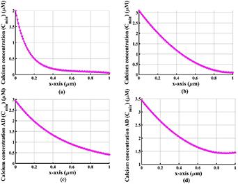
Figure 1. Calcium profile for the normal and AD-affected cells with fuzzy lower condition. |
Moreover, rapid decline in calcium concentration from an initially elevated level signifies a substantial initial calcium presence that decreases progressively along the x-axis. Experimental results indicate that in Alzheimer's circumstances, the buffer quantity drops to 30%-35% [48]. In this work, Alzheimer's-affected cells are given a buffer concentration of ${\text{ }}B = 0.3{B_0} - 0.35{B_0}$. Figures 1(c) and (d) demonstrates the cells with the high calcium concentration when affected by AD. The Alzheimer-affected cell is exacerbated by this loss in buffer, which raises the concentration of calcium. Because of the abnormally high ER calcium activities linked to AD, it is anticipated that the values for calcium flux via the ER are greater than normal.
The loss of buffering capacity exacerbates calcium accumulation within the cell, leading to abnormally elevated intracellular calcium levels. Furthermore, due to enhanced ER calcium dysregulation associated with AD, the calcium flux through the ER is assumed to be higher than that of healthy cells.
Figures 2(a) and (b) demonstrate the variation in calcium along the x-axis for the upper condition. Cytosolic calcium is highest at the source and attains the background level of concentration as it fades down the x-axis. Furthermore, we discovered that the buffer's presence lowers the calcium concentration because it binds calcium that is free and lessens the amount of free calcium ions in the cytosol. Figures 2(c) and (d) exhibit a higher level of calcium abundance for both the approaches with lower and upper conditions respectively. Consequently, it can be concluded that the buffer and ER are important for preserving the level of cytosolic calcium concentration, the health of nerve cells depends on it [49]. Furthermore, the findings show that the concentration of calcium is maximum close to the source and subsequently progressively drops under different circumstances. This pattern suggests that calcium levels peak closest to the point of origin, diminishing as the distance increases, regardless of the specific circumstances being examined. Increased calcium concentrations near the plasma membrane have been linked to increased activation of VGCCs, which are thought to be dysregulated in Alzheimer's. Prolonged VGCC opening causes excessive calcium influx, which amplifies cytosolic calcium accumulation, similar with the higher concentration profiles observed in the Alzheimer's case.
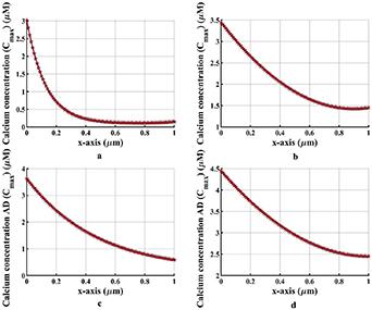
Figure 2. Calcium profile for the normal and AD-affected cells with fuzzy upper condition. |
The findings show that whereas ER-related dynamics are essential for controlling calcium release and redistribution, buffering mechanisms lessen variations in calcium concentration, promoting system stability.
According to the fuzzy boundary conditions principles, a crisp solution is one that is situated between the range of the upper and lower bound of a fuzzy solution [26]. Figures 3(a) and (b) elaborate on the nature of calcium concentration for the deterministic values as well as linguistic values for upper and lower cases. Comparably, the spatial distribution of calcium concentration under typical circumstances exhibits a similar pattern, as demonstrated in the work of [8]. Furthermore, figure 3(a) follows the anticipated pattern, while figure 3(b) deviates from the fuzzy rules in that at the place of the source, the calcium content is elevated, and as one gets further away, it decreases. During the linear transformation strategy, the crisp solution usually lies between the upper and lower boundaries, as previously mentioned. However, with the undetermined fuzzy coefficient approach, the initial values conform to the expected range, but as the distance increases, they deviate from these bounds. The deviation suggests that to retain the predicted behavior within the given range, the linear transformation approach is preferable over the indeterminate fuzzy coefficient approach.
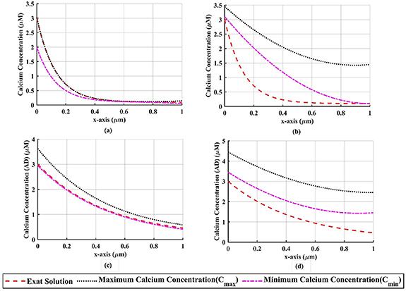
Figure 3. Calcium concentration profiles for normal and Alzheimer's disease (AD)-affected cells, computed using both approaches, showing the influence of fuzzy lower and upper boundary conditions. |
In Alzheimer's affected cells, calmodulin levels are seen to be significantly lower in certain regions of neurons [1]. Research has indicated that cells affected by AD have markedly increased ER and buffer activity. It is noted in figures 3(c) and (d) that the buffer levels drop and unbound calcium concentration levels increase. Sustained intracellular calcium elevation above healthy resting levels impairs synaptic signaling and activates calcium-dependent neurotoxic pathways, eventually leading to neuronal degeneration, resulting in cell death and loss. AD, the most prevalent kind of dementia, is characterized by memory loss and language impairments, which are caused by the death of brain cells and the shrinking of the brain. So, it is necessary to keep free calcium levels stable, which supports the efficient operation of the calcium signaling pathway in neuronal cells.
Figure 4 thoroughly investigates the spatial irregularities of calcium abundance along the x, y-directions amid buffering agents and ER. The figure offers a comparative evaluation of two modeling approaches, highlighting their impact on the resulting calcium distribution. Notably, the linear transformation technique consistently results in lower calcium concentrations at both lower and higher boundary conditions. Calcium levels decrease gradually in both techniques before stabilizing at baseline levels. This decline becomes more apparent as the distance to the calcium source rises in both spatial directions. The figure is an important visual tool because it provides a thorough two-dimensional spatial view of calcium dynamics, which is required for studying cellular calcium signaling pathways and their larger implications for physiological processes. The graphic sheds light on calcium control and its consequences for cellular health by contrasting two separate modeling methodologies. Elevated calcium levels, which are frequently related to cellular toxicity, can cause apoptosis, leading to neurological diseases like Alzheimer's. Interestingly, the indeterminate fuzzy coefficient technique predicts greater calcium concentrations under both boundary conditions, which may provide a more nuanced understanding of calcium's involvement in cellular homeostasis and disease development.
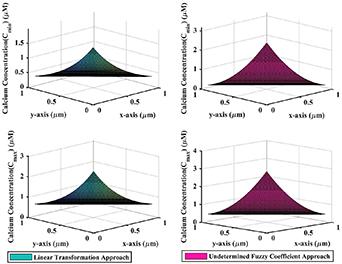
Figure 4. Reconstructed two-dimensional calcium concentration profiles using the similarity solution employing the converted spatial variable. |
When compared to the precise solution, the error values in the linear transformation approach (LTA) gradually decrease down the x-axis, showing improved convergence, as seen graphically in figure 5. On the other hand, the undetermined coefficient approach (UCA) indicates a divergence from the precise answer with a rising trend in error values down the x-axis. This trend shows that, in contrast to UCA, the LTA approach effectively models such error-minimizing behavior. Also, the above figure illustrates the changes in calcium concentration for both the approaches. When comparing the LTA approach to the precise solution, the inaccuracy in calcium concentration reduces along the x-axis, indicating a more realistic depiction of calcium dynamics, such as in brain signaling. This shows that LTA more accurately mimics the regulatory feedback processes that preserve calcium homeostasis. On the other hand, the UCA approach exhibits growing error values with the x-axis, indicating that it fails to accurately capture the fluctuations and spatial variations in calcium concentration. As a result, the LTA method is more in line with the physiological behavior of calcium regulation in biological systems, where precise regulation is necessary for the proper functioning of cells.
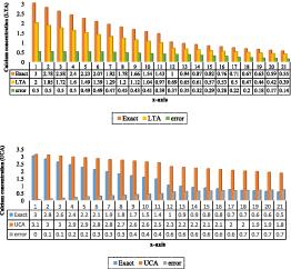
Figure 5. Error analysis of both approaches compared to the exact solution. |
The fluctuation in calcium concentration as x varies is seen in figure 6 for both the indeterminate coefficient and linear transformation techniques. The calcium concentration values for the linear transformation approach exhibit a discernible drop as x grows, suggesting a sensitivity to variations in x. On the other hand, the calcium concentration values obtained using the indeterminate coefficient technique show fewer variations. Consequently, there is an increasing disparity in the predicted calcium concentration as x fluctuates, as seen by the error values between these two approaches increasing gradually with changes in x.
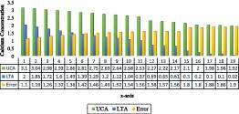
Figure 6. Error analysis comparison between the undetermined coefficient approach and linear transformation approach. |
This shows that the linear transformation approach is more suited for simulating calcium homeostasis because it responds more accurately to changes in x, which may reflect external stimuli or internal circumstances. The undetermined coefficient approach is less sensitive to changes in x, possibly resulting in losing important information about calcium flow. The improved performance of the linear transformation approach enhances our understanding of calcium-dependent cellular mechanisms and allows for more reliable predictions in experimental and clinical settings. Precisely modeling of calcium dynamics is critical for interpreting cellular responses and designing therapeutic strategies.
8. Homotopy Analysis Method (HAM) for convergence analysis
The convergence-control parameter determines the rate of convergence of the equation approximation. There are multiple approaches to get $\hslash ^{^{\prime} }$ value for a specific order of HAM approximation series solutions that produce a highly precise density [50].
Considering the boundary value problem
$\begin{equation}\frac{{{\text{d}^2}C}}{{\text{d}{X^2}}} - {p_1}C + {q_1} = 0.\end{equation}$
With the boundary conditions
$\begin{equation*}\tilde C\left( 0 \right) = \left[ {2 + \alpha ,3.5 - 0.5 \alpha } \right],\,\,\,\tilde C\left( 1 \right) = \left[ { \alpha ,1.5 - 0.5 \alpha } \right].\end{equation*}$
First estimate for the approximation is represented as follows
$\begin{align}&{\underline {C}} _{\alpha ,0}\left( \chi \right) = \left( {2 + \alpha } \right) + \left( \alpha \right)\chi ,\\[-6pt]\end{align}$
$\begin{align}& {\bar C_{ \alpha ,0}}\left( \chi \right) = \left( {3.5 - 0.5 \alpha } \right) + \left( {1.5 - 0.5 \alpha } \right)\chi .\end{align}$
The mth order deformation equation can be expressed as follows for ${\text{ }}m \unicode{x2A7E} 1$ [50-52]:
$\begin{equation}{{\underline {L}} _2}\left[ {{{{\underline {C}} }_m}\left( {\chi ; \alpha } \right) - {\xi _m}{{{\underline {C}} }_{m - 1}}\left( {\chi ; \alpha } \right)} \right] = \hslash {R_m}\left( {{{ {\underline {\boldsymbol{C}} } }_{m - 1}}\left( {\chi ; \alpha } \right)} \right),\end{equation}$
$\begin{equation}{\bar L_2}\left[ {{{\bar C}_m}\left( {\chi ; \alpha } \right) - {\xi _m}{{\bar C}_{m - 1}}\left( {\chi ; \alpha } \right)} \right] = \hslash {R_m}\left( {{{ {\overline {\boldsymbol{C}} } }_{m - 1}}\left( {\chi ; \alpha } \right)} \right),\end{equation}$
where $\begin{align}{R_m}\left( {{{ {\underline {\boldsymbol{C}} } }_{m - 1}}\left( {\chi ; \alpha } \right)} \right)& = {\underline {C^{^{\prime}\! ^{\prime} }} _{ \alpha ,m - 1}}\left( {\chi ; \alpha } \right) - u{\bar C_{ \alpha ,m - 1}}\left( {\chi ; \alpha } \right)\nonumber\\ &\quad + v\left( {1 - {\xi _m}} \right),\end{align}$
$\begin{align}{R_m}\left( {{{ {\overline {\boldsymbol{C}} } }_{m - 1}}\left( {\chi ; \alpha } \right)} \right)& = {\bar C_{ \alpha ,m - 1}}\left( {\chi ; \alpha } \right) - u{{\underline {C}} _{ \alpha ,m - 1}}\left( {\chi ; \alpha } \right)\nonumber\\ &\quad + v\left( {1 - {\xi _m}} \right).\end{align}$
Let us consider, ${\text{ }}{{{L}}_{{i}}} = \frac{{\text{d}}}{{{\text{d}t}}}{\text{ }},{{ i}} = 1,2$
Once the initial approximation has been determined, the following terms can be added to the HAM series solutions using the iteration formulae from equation (39 ) and as follows:
$\begin{align*}{{\underline {C}} _{ \alpha ,1}}\left( X \right) = \hslash \frac{{{X^2}}}{2}\left\{ { - u\left( {2 - \alpha } \right) + v} \right\} - \hslash \frac{{{X^3}}}{6}\left\{ {u\left( {0.5 - 0.5 \alpha } \right)} \right\},\end{align*}$
$\begin{align*}{\bar C_{ \alpha ,1}}\left( X \right) = \hslash \frac{{{X^2}}}{2}\left\{ { - u\left( {0.5 + 0.5 \alpha } \right) + v} \right\} - \hslash \frac{{{X^3}}}{6}\left\{ {u\left( {0.1 - 0.1 \alpha } \right)} \right\}.\end{align*}$
To determine the convergence of a series solution for a given feasible value of h, successive approximation terms are monitored for degradation. The truncated HAM solution is deemed convergent when the difference between two successive orders fulfills
$\left\|U_{N+1}-U_{N}\right\|<\epsilon,$
where $ \epsilon $ is the specified tolerance.The error associated with the HAM approximation is quantified through the residual error, obtained by substituting the truncated series solution into the original governing equations. The residual error norm is defined as:
$\begin{equation*}{\varepsilon _N} = \left| {\left| {\mathcal{L}\left( {{u_N}} \right) - N\left( {{u_N}} \right)} \right|} \right|,\end{equation*}$
where ${u_N}$ is the $N$th-order HAM approximation, while $\mathcal{L}$ and $N$ represent linear and nonlinear operators, respectively.The appropriate selection of the convergence-control parameter $\hslash $ guarantees the convergence of the HAM solution. According to the standard HAM theory, the solution series converges if $\hslash $ falls within an admissible range, which can be found via residual error analysis or $\hslash $-curves. This ensures that the solution produced is legitimate and stable.
In a similar manner, there are more terms that we may locate. The dependence of the sequential representation on $ \alpha ,x$, and the convergence criterion $\hslash $ is evident. The solution's convergence region provided by the Homotopy analysis approach can be changed by varying the convergent control parameter [51, 52]. We have drawn the convergence curve for several values of a, while maintaining x fixed at 0.5, to illustrate the convergent domain. $ \alpha $ values are taken into consideration in the range of 0-1. For many a-cuts ${\text{ }}\left( {x = 0.5} \right)$, where $ \alpha $ is a real value between 0 and 1, we have drawn the convergence curve. To illustrate the convergence domain, this is done.
Figure 7 shows how calcium concentration profiles converge under fuzzy lower and upper boundary conditions at various $ \alpha $ values. As $ \alpha $ grows from 0.2 to 1, the gap between the bottom and higher solutions gradually diminishes, indicating effective control and reduced uncertainty. At ${\text{ }} \alpha = 1$, both solutions converge to the crisp solution, demonstrating the consistency and stability of the fuzzy formulation. Moreover, the calcium concentration profiles along $h$ for various fuzzy levels $ \alpha $ are displayed in the above figures. Concentration rises with $ \alpha $ in the first figure and falls with $ \alpha $ in the second, showing opposing boundaries of uncertainty. In both situations, the concentration of calcium progressively decreases with distance and approaches zero near the boundary.
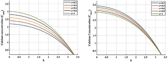


Figure 7. Convergence control for fuzzy lower and upper conditions. |
The HAM solution's convergence depends on the auxiliary parameter ${\text{ }}h$, which is crucial for stability and convergence. In the present study, the convergence behavior of the solution series is used to determine the permissible range of ${\text{ }}h$. The HAM series converges rapidly within this range, however values outside of this range result in divergence or oscillations.
9. Conclusions
This study investigates calcium concentration by employing a two-dimensional computational model, highlighting that calcium levels are affected by key parameters such as buffer and ER. While the ER has a huge calcium reservoir, buffers primarily aid in reducing calcium levels, as elevated levels of calcium have been linked to cellular damage and neurological diseases such as AD. The findings indicate that the levels of cytosolic calcium concentration are profoundly influenced by each of these parameters. To quantitatively estimate the amount of calcium circulation in cells with and without AD, a FBVP was formulated. The proposed model was solved by distinct two approaches such as a linear transformation approach and an undetermined fuzzy coefficient approach.
The chosen fuzzy modeling approaches are especially good for solving boundary value problems with fuzzy parameters since they are flexible and easy to understand. They provide a direct analytical approach to fuzziness inside the system, eliminating the necessity for defuzzification and thereby maintaining the uncertainty framework throughout the solution process. By converting the fuzzy system into a series of precise problems at different a-levels, they provide both computing efficiency and clarity. These attributes render the selected methodologies exceptionally suitable for preserving the mathematical framework and precisely delineating the propagation of uncertainty in fuzzy differential systems.
The outcomes are obtained by applying boundary conditions that, under the given environment, closely resemble the properties of a normal neuronal cell in the brain, demonstrating that free calcium concentrations are much greater in Alzheimer's-affected cells than in healthy ones. This elevated calcium concentration increases the risk of cellular toxicity, which potentially leads to the formation of amyloid plaques and neurofibrillary tangles. The comparison between the two approaches highlights that the linear transformation is more effective in this context, providing explicit analytical solutions that are useful for theoretical analysis and understanding the problem's behavior. Also, it effectively manages the fuzziness in boundary conditions and leading to more accurate and precise solutions. The error analysis of calcium concentration for different methodologies is shown, demonstrating how calcium levels varied between approaches. This difference has important ramifications for neurological conditions like AD since high calcium concentrations are known to negatively impact on neuronal cells, which may aid in the onset and progression of these conditions.
Moreover, HAM is used to assess convergence behavior, assure numerical stability, validate the technique, and increase computing efficiency. This approach satisfies both minimum and maximum criteria by efficiently generating approximate solutions and providing a simple means of controlling the convergence zone for FBVPs. Adopting a triangular fuzzy number allows HAM to produce results that are consistent with fuzzy number characteristics. However, a FDE framework provides valuable insight, it presents limitations especially when the computational model has large scale or systems with high dimensions. The study underscores the significant influence of the aforementioned characteristics in a fuzzy environment, eventually in the context of neurological disorders. The metrics probably relate to certain conditions or factors that affect these cells, which is fundamentally beneficial for scientists and researchers. This study is solely computational in nature, focusing on the methodological examination of fuzzy solution techniques for calcium diffusion models; experimental or clinical validation is outside the scope of the present work and is intended as a future research area.