

1. Introduction
Quantum entanglement, a cornerstone of quantum information, is crucial for understanding the behavior of quantum many-body systems and the nature of gravity [1-8]. Over recent decades, entanglement has propelled advancements in quantum computation [9], uncovered novel quantum phases [10-12], and shed light on quantum gravity phenomena [13-15]. Quantitatively, various entanglement measures, such as von Neumann entropy (entanglement entropy), Rényi entropy, mutual information, and negativity, have been introduced to quantify the entanglement structure [1] and provide an intuitive picture of how entanglement distributes. However, these measures are insufficient to fully characterize quantum entanglement, as each has its strengths and weaknesses in capturing different aspects of quantum entanglement. For example, entanglement entropy is defined for pure state entanglement, whereas for mixed states, negativity is often used. However, negativity can be zero even if the state is entangled [16]. Mutual information can detect mixed state entanglement but struggles to distinguish between quantum entanglement and classical correlations, a distinction where entanglement entropy excels. Furthermore, as single numbers, they also fail to reveal much information about the eigen properties of the density matrix of the subregion $A$ (denoted as $\hat{\rho}_A$), i.e. entanglement spectrum and entanglement wave function (Schmidt vectors) [11, 17, 18].
Chen and Vidal first put forward an entanglement quantity called 'entanglement contour' [19] that can be regarded as the fine structure of entanglement distribution in real space. More precisely, the entanglement entropy $S(A)$ between a subregion $A$ and its complement $\bar A$ is decomposed as the sum of entanglement contour $s(i)$ over all sites, expressed as $S(A) = \sum_{i \in A} s(i)$. Since then, the contour function $s(i)$ has been explored in various contexts: fractal lattice [20], Gaussian states [19], conformal field theory (CFT) [21, 22], geometric construction in the AdS/CFT correspondence, and partial entanglement entropy derived by the additive linear combination of subset entanglement entropy [23]. The extension to the $n$th order Rényi entropy $S_n(A)$, defined as $S_n(A) = \frac{1}{1-n}\mathrm{ln}\,\mathrm{tr}\hat{\rho}_A^n$, has also been explored by introducing the $n$th order Rényi contour $s_{n}(i)$ [19, 21, 24, 25], as below:
$equation*$
In this work, we significantly expand the zoo of entanglement quantities and uncover a deeper understanding of quantum entanglement by introducing the hyperfine structure of entanglement. Specifically, we precisely decompose the fine structure of entanglement $s_{n}(i)$, into contributions from particle-number cumulants, i.e. $s_n(i) = \sum_{k = 1}^\infty h_{n;k}(i)$ defined in equation (1 ). We rigorously prove that the hyperfine structure, represented by $h_{n;k}(i)$, is an exotic entanglement quantity with several universal properties, including additivity, normalization, exchange symmetry, and local unitary invariance, making the hyperfine structure physical and meaningful just like other quantum informative measures. We then apply this quantity to the following three distinct physical contexts, demonstrating plentiful findings.
First, in a Fermi gas, we find that $s_{n}(i) \approx h_{n;2}(i)$, with all $h_{n;k}$ for $k \gt 2$ being suppressed. Using this simplified relation, we establish the connection between $h_{n;2}$ and mutual information, showing that $h_{n;2}$ negatively contribute to the mutual information. We also show that, for the vacuum of a $(1+1)$D CFT with a conserved $U(1)$ charge, the leading hyperfine component $h_{n;2}(x)$ and the entanglement contour $s_n(x)$ share the same universal spatial profile, and hence are proportional up to a theory-dependent constant. Second, from a holographic perspective, the hyperfine structure of entanglement unveils a finer subregion-subregion duality in the bulk reconstruction. Specifically, we demonstrate that the hyperfine structure of holographic refined Rényi entropy is dual to the density-density correlator in the boundary subregion. Surprisingly, for a given boundary subregion, the bulk extremal surfaces associated with refined Rényi entropy can extend beyond the entanglement wedge determined by entanglement entropy. It indicates that the holographic dual of refined Rényi entropy and its hyperfine structure can be utilized to construct more information outside the entanglement wedge. Third, by investigating a prototypical (2+1)D lattice model, we numerically observe significant distinctions in the hyperfine structure across parameter regions, such as trivial mass gap, topological gap (supporting edge states and nonzero bulk Chern number), Dirac critical point, and Fermi surface. This hyperfine structure, based on local measurement, is experimentally accessible, such as through a quantum point contact (QPC). We conclude by discussing several future directions based on these findings.
2. Definition and properties
Focusing on general Gaussian states for free fermions with conserved charge, to introduce the hyperfine structure of entanglement, denoted as $h_{n;k}(j)$, we precisely decompose the $n$th order Rényi contour $s_{n}(j)$ at site $j$ in subsystem $A$ according to the contribution from all particle-number cumulants (details in the supplementary material (SM) [26] section-I): 1 ). Interestingly, this process is reversible when a cutoff is applied, as we can use information about $s_n(j)$ to reconstruct the set of $C_k(j)$.
$align$
where $\beta_k(n)$ is non-zero only for even $k$. $\beta_k(n) = \frac{2}{n-1}\frac{1}{k!}\left(\frac{2\pi {\mathrm{i}}}{n}\right)^k\zeta\left(-k,\frac{n+1}{2}\right)$, with $\zeta\left(-k,\frac{n+1}{2}\right)$ as the Hurwitz zeta function [27]. For instance, $\beta_2(2) = \frac{\pi^2}{4}$, $\beta_4(2) = -\frac{\pi^4}{192}$, and so forth. Here, the density of cumulant $C_k(j)$ on site $j$ is defined as $align$
where $\hat n_j$ represents the particle-number operator at site $j$, $\hat N_A$ is the total particle-number operator for the subsystem $A$, and $\lambda$ is a real number. We observe that $C_k(j)$ corresponds to the $2k$-point correlation function. The first non-zero term $C_2(j)$ simplifies to $C_2(j) = \sum_i \langle \hat n_i \hat n_j\rangle - \langle \hat n_i \rangle\langle \hat n_j\rangle$. The complete set of $C_k(j)$ with even $k$ can be utilized to obtain the complete set of $s_n(j)$ based on equation (Moreover, the hyperfine structure $h_{n;k}(j)$ defined in equation (1 ) exhibits several universal properties as an quantum information quantity: (i). Additivity. For $i,j\in A$, $h_{n;k}(i) + h_{n;k}(j) = h_{n;k}(i \cup j)$. (ii). Normalization. The sum of $h_{n;k}(j)$ over all sites in $A$ equals the particle-number cumulant $C_k$, specifically, $C_k = \sum_j h_{n;k}(j)/\beta_k(n)$. Here, $C_k$ is defined as $C_k \equiv (-{\mathrm{i}}\partial_{\lambda})^k \ln \chi(\lambda, \hat{N}_A) \big|_{\lambda = 0}$, with the generating function $\chi(\lambda, \hat{N}_A) \equiv \langle \exp({\mathrm{i}}\lambda \hat{N}_A) \rangle$. (iii). Exchange symmetry. If $\hat{T}$ represents a symmetry of the reduced density matrix $\hat{\rho}_A$ and satisfies $\hat{T}\hat{\rho}_A\hat{T}^{\dagger} = \hat{\rho}_A$, and $\hat{T}$ exchanges site $i$ with site $j$, then $h_{n;k}(i) = h_{n;k}(j)$. (iv). Local unitary invariance. If the quantum state transforms from $|\psi\rangle$ to $|\psi^{^{\prime}}\rangle$ using a unitary transformation $\hat U^X$ acting on a subset $X \subset A$, then $h_{n;k}(j\in X)$ remains the same for both states $|\psi\rangle$ and $|\psi^{^{\prime}}\rangle$. Notably, both $h_{n;k}(j)$ and $C_k(j)$ can be either negative or positive, but $s_n(j)$ must be positive. We also discuss the non-increasing property under local operations and classical communication in SM [26] section-VB.
3. Fermi gas
We begin by applying the hyperfine structure to the $(d+1)$D Fermi gas in continuum spacetime. Our analysis reveals that the summation of all $h_{n;k}$ terms with $k \gt 2$ is significantly suppressed, leading to a simplified exact expression of equation (1 ) as follows (see SM [26] section-II):
$align$
where $align$
Here, $\hat{n}(x)$ represents the particle-number operator at position $x$, and $o(1)$ denotes a term that is negligible compared to 1. This simplified expression is closely connected to the mutual information $I_2(A_1, A_2) \equiv S(A_1) + S(A_2) - S(A_1 \cup A_2)$ between regions $A_1$ and $A_2$ (see figure 1(a)) through the relation: $align$
where $h_{1;2}(x)$ is the hyperfine structure of the combined region $A_1 \cup A_2 = A$. It is evident that the integral of the hyperfine structure contributes negatively to the mutual information between $A_1$ and $A_2$. More intriguingly, by utilizing the entropy and hyperfine structure of subregion $A_1$, we can derive the mutual information $I_2(A_1, A_2)$ without the need to consider any additional properties of $A_2$.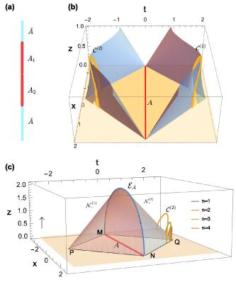
Figure 1. (a) A tripartition of the system to calculate the mutual information $I_2(A_1,A_2)$, where $A_1$ and $A_2$ can be disjoint. In (c) ((b)), the two transparent surfaces are the null hypersurfaces $\mathcal{N}^{(1)}_{\pm} (\mathcal{N}^{(2)}_{\pm})$, intersecting at the RT surface $\mathcal{E}_A$ (the extremal surface $\mathcal{C}^{(2)}$). Discontinuities occur on the null hypersurfaces $\mathcal{N}^{(n\neq 1)}_{\pm}$ due to conical defect and the backreaction from $\mathcal{C}^{(n)}$. These singularities vanish when $n = 1$. For $n \unicode{x2A7E} 2$, the intersections of $\mathcal{N}^{(n)}_{\pm}$ form $\mathcal{C}^{(n)}$, depicted as yellow, green, and orange curves for $n = 2, 3, 4$ respectively. Clusters of $\mathcal{C}^{(n)}$ appear on both sides of $\mathcal{E}_A$, though for clarity, only the clusters on the right are shown in (c). We set $R = 2$. |
To proceed further, we explicitly derive the hyperfine structure in a $(1+1)$D CFT as an example, which is useful in the next section. We consider the action of free Dirac Fermions, given by $ S = \frac{1}{2} \int {\mathrm{d}}^2x \bar \psi\gamma_{\mu}\partial^{\mu}\psi$, where $\psi = (\psi_R,\psi_L)^{\mathrm{T}}.$ The corresponding correlation functions are $ \langle \psi_R^{\dagger}(z)\psi_R(\omega)\rangle = -\frac{1}{2\pi}\frac{1}{z-\omega}$,$\quad \langle \psi_L^{\dagger}(\bar z)\psi_L(\bar \omega)\rangle = -\frac{1}{2\pi}\frac{1}{\bar z-\bar \omega}$. Considering $A$ as an interval with $x\in(-R+\epsilon,R-\epsilon)$ on an infinite line (where $R$ is $A$'s radius and $\epsilon$ is the UV cutoff), we have the dominant hyperfine structure as  . Comparing the known equality $S_n = [\left(1+n^{-1}\right)c/6]\ln\frac{2R}{\epsilon}$, we end up with the value of the central charge $c = 1$, which agrees with the known fact of free Dirac fermions models. Interestingly, we observe that the dominant hyperfine structure $h_{n;2}$ is independent of the UV cutoff, unlike Rényi entropy $S_n$.
$align$
By integrating $s_{n}(x)$ over $A$, we can obtain the Rényi entropy as $$S_n = \int_{-R+\epsilon}^{R-\epsilon} {\mathrm{d}}x s_n(x) \approx[\left(1+n^{-1}\right)/6]\ln\frac{2R}{\epsilon}$$. Comparing the known equality $S_n = [\left(1+n^{-1}\right)c/6]\ln\frac{2R}{\epsilon}$, we end up with the value of the central charge $c = 1$, which agrees with the known fact of free Dirac fermions models. Interestingly, we observe that the dominant hyperfine structure $h_{n;2}$ is independent of the UV cutoff, unlike Rényi entropy $S_n$.4. Holographic duality
From the AdS/CFT correspondence, the entanglement entropy of boundary subregion $A$ can be determined by the extremal surface (homologous to the boundary of $A$) in bulk AdS spacetime, which is called the Ryu-Takayanagi (RT) surface $\mathcal{E}_A$ [13, 28] in figure 1(c). It is natural to ask what the holographic dual of the hyperfine structure is.
In the following we will answer this question by considering the refined Rényi entropy $ \tilde S_n \equiv n^2\partial_n\left(\frac{(n-1)}{n}S_n\right)$, which has been shown to be dual to the cosmic brane in the bulk AdS spacetime [29]. The relation between particle-number fluctuation and Rényi contour in equation (3 ) can be rewritten for the $n$th refined Rényi contour as 7 ) is initially derived from the non-interacting Fermi gas, it can be extended to the vacuum of a $(1+1)$D CFT with a conserved $U(1)$ charge up to a theory-dependent constant, since both the contour function $\tilde{s}_n(x)$ and the local cumulant density $C_2(x)$ share the same universal spatial profile $\frac{1}{R-x}+\frac{1}{R+x}$ (see SM [26] section-IIB for details). Thus, equation (7 ) remains applicable in the large central charge limit, which admits a dual description in terms of classical bulk AdS gravity [30].
$align$
It is crucial to recognize that although equation (To elucidate the holographic dual within the AdS$_3$ spacetime, we employ the Rindler transformation [15]. The fundamental idea of the Rindler transformation is to map the entanglement entropy of a region to the thermal entropy of another region, which can then be associated with the horizon entropy of a hyperbolic black hole. It turns out that the horizon corresponds to the null hypersurfaces $\mathcal{N}^{(1)}_{\pm}$ in the original AdS spacetime, as illustrated in figure 1(c). The intersection of these null hypersurfaces is the extremal surface $\mathcal{E}_A$. It can be shown that the refined Rényi entropy of $\hat{\rho}_A$ is equivalent to the entanglement entropy of the $n$-replica reduced density matrix $\tilde{\rho}_A \equiv \frac{(\hat{\rho}_A)^n}{\mathrm{tr} (\hat{\rho}_A)^n}$ (see SM [26] section-III). Therefore, the intersection of the $n$-dependent null hypersurfaces $\mathcal{N}^{(n)}_{\pm}$ is the holographic dual of $\tilde{S}_n$ in figures 1(b) and (c). Notably, within the entanglement wedge enclosed by the boundary $PMQN$ and $\mathcal{E}_A$, the bulk operators can be reconstructed from the boundary CFT, which is the celebrated subregion-subregion duality in holographic duality [31, 32, 33-36].
Moreover, with the help of the hyperfine structure, we can propose a natural geometric interpretation of the subregion structure in the entanglement wedge and the Rényi entanglement wedge. Explicitly, we use the planes connecting boundary sites to the extremal surfaces $\mathcal{C}^{(n)}$ to slice the extremal surface according to the contour distribution in equation (7 ). This suggests that different segments of the extremal surface are associated with different local contributions to the hyperfine structure. In this sense, the holographic description of Rényi entropy is geometrically refined by the boundary decomposition.
Interestingly, after mapping all extremal surfaces back to the same original Poincaré coordinate system through the inverse Rindler transformation, we find that $\mathcal{C}^{(n)}$ with $n \gt 1$ extends beyond the ordinary entanglement wedge. This suggests that the hyperfine structure is geometrically associated with a region beyond the RT wedge. It is noteworthy that $\mathcal{C}^{(n)}$ with $n \gt 1$ differs significantly from the $n = 1$ RT surface $\mathcal{E}_A$. First, $\mathcal{C}^{(n)}$ is tilted in the time direction and carries a conical defect, manifested as discontinuities in $\mathcal{N}_{\pm}^{(n)}$. Second, $\mathcal{C}^{(n)}$ cannot be obtained from $\mathcal{E}_A$ by ordinary time evolution, since unitary time evolution does not change the entanglement spectrum of a density matrix. We note that the $n \gt 1$ geometry involves a conical singularity, and the physical interpretation of the corresponding Rényi wedge deserves further study.
5. Chern insulators
Next, we investigate the behavior of $s_n(j)$ and $h_{n;k}(j)$ in the $(2+1)$D Chern insulator [37-39]: $\hat{\mathcal{H}} = \sum_{\boldsymbol{k}}\hat c_{\boldsymbol{k}}^{\dagger}H(\boldsymbol{k})\hat c_{\boldsymbol{k}}$, where $ H(\boldsymbol{k}) = (m+\cos {k}_x+\cos {k}_y)\sigma_z+\lambda(\sin {k}_x\sigma_x+\sin {k}_y\sigma_y)-\mu \boldsymbol{I}$, $\sigma_i$ represents the Pauli matrices and $\boldsymbol{I}$ is the $2\times 2$ identity matrix. This Hamiltonian comprises a Zeeman splitting term induced by the mass parameter $m$ and a spin-orbit coupling term with amplitude $\lambda$. The energy gap closes at $ m = \pm 2$, forming a Dirac point respectively at $ \boldsymbol{k} = (0,0)$ and $ \boldsymbol{k} = (\pi,\pi)$. For $m = 0$, the energy gaps close, creating two Dirac points with vanishing density-of-states: one at $ \boldsymbol{k} = (0,\pi)$ and the other at $ \boldsymbol{k} = (\pi,0)$. In the following, we consider four distinct scenarios: (i) trivial mass gap; (ii) topological mass gap (supporting nonzero Chern number and robust edge states); (iii) critical Dirac point; (iv) Fermi surface.
Figure 2 displays the distributions of $s_n(j), h_{n;2}(j), h_{n;4}(j),$ and $h_{n;6}(j)$ for various types of parameters. The four rows correspond to cases of trivial mass gap, topological mass gap, critical Dirac point, and Fermi surface. The four columns represent different terms of the hyperfine structure. Notably, the behavior of $h_{n;k \gt 6}$ resembles that of $h_{n;4}(j)$ and $h_{n;6}(j)$, thus we focus on the first three non-zero terms $h_{n;2,4,6}(j)$.
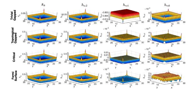
Figure 2. Distribution of $s_n(j)$ and $h_{n;k}(j)$ for different types of parameter regions in a $60\times 60$ lattice model with periodic boundary conditions in both $x$ and $y$ coordinates. Region $A$ contains $30\times 30$ sites. The first row shows the case of a trivial mass gap with $m = 3$ and chemical potential $\mu = 0$, the second row shows the case of a topological gap with $m = 1,\mu = 0$, the third row shows the case of critical point with $m = 0,\mu = 0$, and the last row shows the case of a Fermi surface with $m = 0$ and $\mu = 2/3$. We consider $n = 2$ and $\lambda = 1$ in all cases. The four columns represent the distributions of $s_n(j), h_{n;2}(j), h_{n;4}(j),$ and $h_{n;6}(j)$, respectively. |
Examining the first two columns within each row, we observe that the distribution and magnitude of $s_n(j)$ and $h_{n;2}(j)$ are very similar, indicating that $h_{n;2}$ is dominant in the series $h_{n;k}$. This aligns with previous findings [40] showing a numerical resemblance between the entanglement contour and the density of $C_2$. In addition to this observation, we find more interesting features as follows.
Comparing the distribution of $h_{n;2}(j)$ across the three system types, we note that in cases of mass gap (either trivial or topological) and critical points, $h_{n;2}(j)$ decays more rapidly from the boundary of $A$ to the center of $A$ compared to the Fermi surface case. Upon further investigation, we find that in cases of mass gap (either trivial or topological), $h_{n;2}(j)$ decays exponentially from the boundary to the center. However, in the cases of critical points and Fermi surfaces, $h_{n;2}(j)$ decays according to a power law but with different power law exponents (see SM [26] section-IV).
As equation (1 ) allows for the analysis of contributions from all values of $k$, we investigate the hyperfine structure $h_{n;k}(j)$ for larger $k$ ($k \gt 2$), as depicted in the third and fourth columns, where negative values of $h_{n;k}(j)$ are observed. In the trivial mass gap scenario, for any given $n$ and $k$, the values of $h_{n;k}(j)$ across the entire region $A$ maintain a consistent sign at all sites $j$, with corner and hinge sites sharing the same sign. However, in both the topological mass gap and critical Dirac point cases, the sign of $h_{n;k}(j)$ at corner sites may differ from that at hinge sites. In this way, we can distinguish the case of trivial mass gap from topological mass gap as well as critical point.
From the distribution of the hyperfine structure in figure 2, the behavior of the topological phase is similar to the critical point. To further detect the topological edge modes, we vary the parameter $m$ across different phases using the partition scheme shown in the upper-right of figure 3(a), where the $y$-axis is an open boundary and the $x$-axis is periodic. We compute $h_{n;k}$ from the edge of region $A$ as a function of $m$, denoted by $ h_{n;k}(m;{k}_x) = \, h_{n;k}(m;{k}_x,y\in \partial A)$, where ${k}_x$ is the momentum quantum number along the $x$-axis and $\partial A$ are the sites near the boundary cut between $A$ and $\bar A$. To ensure a fair comparison and mitigate variations in magnitude, we normalize boundary $h_{n;k}$ by its maximum as $h_{n;k}(m;{k}_x) / \max h_{n;k}(m;{k}_x)$. This normalization process is applied uniformly to all ${k}_x$.
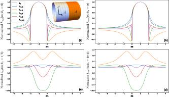
Figure 3. Normalized $h_{n;k}(m; k_x)$ as a function of $m$: (a) $k_x = 0$, (b) $k_x = \pi$, (c) $k_x = \pi/3$, and (d) $k_x = 4\pi/3$. We set $n = 2$ and $\lambda = 1$ for generality. |
We observe that most of the normalized $ h_{n;k}(m;{k}_x)$ are randomly distributed, as shown in figures 3(c) and (d) for $k_x = \pi/3$ and $k_x = 4\pi/3$, except for those with ${k}_x = 0$ and ${k}_x = \pi$. For these special cases, as seen in figures 3(a) and (b), $h_{n;k}(m;{k}_x)$ with different $k$ converge to a single curve and reach their maximum values for $m$ values in the intervals of $(-2,0)$ and $(0,2)$. The emergence of this scaling law within the topological mass gap regions, namely $m\in(-2,0)\cup (0,2)$, indicates the existence of critical edge states and a fundamental $1/2$ mode in the entanglement spectrum. This $1/2$ mode represents the most entangled and correlated mode for $h_{n;k}$ across all values of $k$ and corresponds to the edge states in lattice fermion models. It is essentially the Einstein-Podolsky-Rosen pair that contributes the maximum entanglement. In summary, these distribution properties highlight the different features of a mass gap, a critical Dirac cone, and a Fermi surface, and they reveal a universal scaling behavior in the presence of topological edge states. These discussions can be generalized to a wider class of systems, including other Chern insulators and those with symmetry-protected topological order.
6. Experiment
In this part, we will provide a promising experimental setup to measure the hyperfine structure of the entanglement. The density of particle-number cumulant in equation (2 ) can be simplified as a function of two different cumulant generating functions with different ways of partition (see SM [26] section-V)
$\begin{align} C_k\left(l\right) = \left(-{\mathrm{i}}\partial_{\lambda}\right)^{k-1} \left\{\frac{\left[\chi\left(\lambda,\mathcal{N}_A\right)-\chi\left(\lambda,\mathcal{N}_{A}-1;l\right)\right]}{\chi\left(\lambda,\mathcal{N}_A\right)} \frac{\mathrm{e}^{{\mathrm{i}}\lambda}}{\mathrm{e}^{{\mathrm{i}}\lambda}-1}\right\}\bigg{|}_{\lambda = 0}, \end{align}$
where $\chi(\lambda,\mathcal{N}_{A}-1;j)$ is the cumulant generating function of region $A^{^{\prime}}$ with the $\mathcal{N}_A$ sites, which is a region obtained by removing site $j$ from the original region A. The key observation is that the cumulant generating function $\chi(\lambda,\mathcal{N}_A)$ and $\chi(\lambda,\mathcal{N}_{A}-1;l)$ can be obtained by measuring the cumulants in specific partition configurations based on the QPC method. $\chi(\lambda,\mathcal{N}_A)$ corresponds to the bi-partition shown in the left figure of figure 4 and $\chi(\lambda,\mathcal{N}_{A}-1;l)$ corresponds to the partition arrangement illustrated in the right figure of figure 4, where $A$ and $B$ are not simply connected spaces. The subregion $A$ in the right figure corresponds to the outcome of removing site $j$ from the left subregion $A$, with site $j$ now becoming part of subregion $B$. To mitigate interference within the different parts of $A/B$, we establish additional channels connecting them, positioned above and below the setting. Based on these QPC settings, we can reconstruct the cumulant generating function by measuring the former a few dominant cumulants. To be more precise, considering that the Taylor expansion$\chi(\lambda,\mathcal{N}_A) = \sum_{k = 0}^{\infty} C_k\frac{\lambda^k}{k!}$ centering at $\lambda = 0$, we can reasonably approximate $\chi(\lambda,\mathcal{N}_A)$ by determining the first few terms of the cumulants while the higher-order terms make negligible contributions. These cumulants are experimentally observable in the scheme shown in the left figure of figure 4 as demonstrated in previous studies [17]. These methods can also naturally be applied to the second scheme shown in the right figure of figure 4. Hence, $\chi(\lambda,\mathcal{N}_A)$ and $\chi(\lambda,\mathcal{N}_{A}-1;l)$ can be approximately determined experimentally, which means that $C_k(l)$ can also be obtained using previous experiment methods.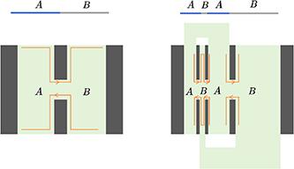


Figure 4. Quantum point contact settings of two types of partition. The left figure corresponds to the bi-partition of $\chi(\lambda,\mathcal{N}_A)$ and the right one corresponds to the partition way of $\chi(\lambda,\mathcal{N}_{A^{^{\prime}}};l)$. |
7. Conclusions and discussions
In this work, we proposed a novel entanglement quantity, termed the hyperfine structure of entanglement $h_{n;k}(j)$, by decomposing the fine structure and Rényi contour into contributions from different particle number cumulants. The hyperfine structure exhibits several universal properties, including additivity, normalization, exchange symmetry, and local unitary invariance, making the hyperfine structure physical and meaningful just like other quantum informative measures. We provided some preliminary and prototypical examples of applications. In a Fermi gas, the hyperfine structure can be analytically expressed as a simple formula, revealing its direct relationship with mutual information. Furthermore, in (1+1)D CFT, the hyperfine structure was shown to be independent of the UV cutoff, demonstrating its robustness as a measurement in field theory. In the context of the AdS/CFT correspondence, we derived the holographic extremal surface for the refined Rényi entropy and established its connection to the hyperfine structure by slicing the extremal surface. This bridges the gap between the holographic duality of Rényi entropy and the cosmic brane description. In addition, we introduced the notion of the Rényi entanglement wedge, which can extend beyond the entanglement wedge, and might provide new framework for bulk reconstruction in the AdS/CFT correspondence. For Chern insulators, we demonstrated that the hyperfine structure can distinguish different parameter regions. Specifically, it can differentiate between topological gapped states and trivial gapped states, which are inaccessible using either the Rényi entropy or fine structure alone. This capability highlights the hyperfine structure as a powerful tool for probing topological phases. Experimentally, we proposed an alternative experimental protocol based on QPCs, similar to previous measurements [17]. The density-density correlator in equation (1 ) can also be measured using atomic quantum gases [41] and trapped ions [42]. These experimental setups also allow us to access the entanglement spectrum and other information about quantum systems.
Our results not only advanced the understanding of entanglement structures in quantum systems but also connected concepts across condensed matter physics, quantum information, and holography. By combining the hyperfine structure of entanglement with other quantum information concepts, such as von Neumann entropy, mutual information, negativity, relative entropy and more, the study of the hyperfine structure will enrich our understanding of quantum entanglement, quantum gravity, and quantum computation. Theoretically, we identify several promising theoretical directions for future study: (i) discuss more general application of the hyperfine structure in the domain of quantum information; (ii) extend the discussions on the hyperfine structure to correlated models, i.e. emergent fermionic spinons; (iii) explore the connection between the inclined extremal surface and the emergent tension in the holographic dual of $\tilde h_{n;2}(j)$, and study bulk reconstruction and surface growth in terms of the Rényi entanglement wedge in the AdS/CFT correspondence; (iv) investigate how the Rényi contour changes under measurement-based operations in quantum computations.