

1. Introduction
General relativity (GR) is the most successful theory for gravity. From weak gravity like the Cavendish experiment to strong gravity involving black holes, from stationary gravity like our Solar System to violent gravity like binary black hole mergers, all experiments support GR up to current experiment accuracy. However, theoretically we still believe GR may break down in some situations. This is due to the contradiction between GR and quantum mechanics on the first hand. Since matter is quantum in first principle and the gravitational field is related to matter through an Einstein equation. On the second hand, GR predicts singularity which means GR breaks down itself.
In the current paper we focus on the singularity problem. Including gravitational wave detections and black hole shadow observations, more and more observations indicate that black holes exist in the Universe. Theoretically black holes can be understood as an event horizon, or more mathematically be understood as a trapping region. That is to say the nature permits that the trapping region exists without singularity. Since Penrose's singularity theorem reports that GR allows the trapping region to result in singularity, a black hole without singularity must violate GR [1]. Black holes without singularity are called regular black holes which have been widely studied in the literature [2-4]. Among regular black holes, there is one category where the black hole is followed by a white hole in the spacetime [5].
Several works have investigated the possible observations of a black hole followed by a white hole [6-8]. In the current paper we ask another possibly observational question: how much time is needed for an object to travel from the black hole to the followed white hole? If this time is too long, even longer than the Universe's age, this kind of spacetime model is very possibly unrealistic. Otherwise, the traveled objects from a black hole to the followed white hole may be observed in our Universe.
More specifically we consider spherical symmetric spacetimes. We define the proper time of the world line connecting the event horizon of the black hole and the event horizon of the white hole as the transfer time from the black hole to the white hole.
In the next section we set up the theoretical framework to calculate the transfer time from the black hole to the white hole. The Schwarzschild type regular black hole models are studied there also. Following that, we study Reissner-Nordstromöm (RN) type models in section 4 and Hayward type black holes in section 5 . We find that the behavior of the transfer time is qualitatively different for these three kinds of models. Finally we conclude this paper in the last section with some discussions.
2. Transfer time from black holes to white holes
The metric of a spherical symmetric spacetime can be expressed as 1 ) is independent of time, the geodesic equations reduce to
$align$
where f and g are functions of t and r and dΩ2 is the line element of a standard sphere. When the metric ($align$
$align$
$align$
where $\phi$ is the rotation direction of the moving object in the spacetime, L and E are its conserved angular momentum and energy. More specifically, the physical meaning of parameter E relies on the asymptotic notions of the spacetime in question. In the current work we have considered all possible values of parameter E, and our regular black hole catalogs do not depend on the detail of the physical meaning of parameter E.Corresponding to the spherical symmetry of the spacetime, we consider a radial direction time-like geodesic connecting the event horizon of the black hole and the event horizon of the white hole. So L = 0. We define the transfer time as the proper time from the geodesic intersection point A on the event horizon of the black hole to the intersection point B on the event horizon of the white hole 4 ), the transfer time can be specified as
$align$
More precisely we use the trapping region to define the black hole and use an anti-trapping region to define the white hole. Instead of the event horizon mentioned above, we use the boundary of the black hole and white hole to determine the aforementioned A and B. According to ($align$
where $E\unicode{x2A7E} 0$ is the conserved energy along with the time-like geodesic.In standard GR, the metric (1 ) reduces to the Schwarzschild metric. If we neglect the GR violation region and glue a set of Schwarzschild spacetimes at r = 0, we get a simplified black hole-white hole transition spacetime [8]. For this spacetime, we have the transfer time
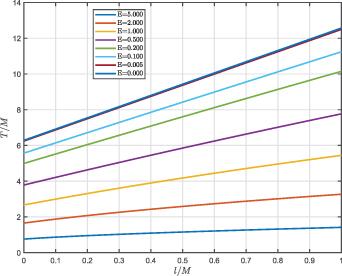
$\begin{align} T& = 2\int_0^{2M}\sqrt{\frac{r}{2M+r\left(E^2-1\right)}}\mathrm{d}r\nonumber\\ & = \left\{\begin{matrix}2M\left[\frac{\pi-2\arcsin E}{\left(1-E^2\right)^{3/2}}-2E/\left(1-E^2\right)\right]\text{if }0\unicode{x2A7D} E\unicode{x2A7D} 1\\[4pt] \kern-8pt 4M\left(E-\frac{\textrm{arcsinh}\sqrt{E^2-1}}{\sqrt{E^2-1}}\right)/\left(E^2-1\right)\text{if }E\unicode{x2A7E} 1 \end{matrix}\right.,\end{align}$
where M is the mass parameter of the Schwarzschild spacetime. We plot this transfer time in figure 1.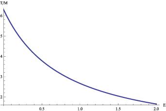
Figure 1. The black hole-white hole transfer time for a simplified black hole-white hole transition spacetime through gluing two Schwarzschild metrics at r = 0 [8]. |
For regular black hole spacetimes, the black hole region is typically followed by a white hole region. The black hole-white hole transfer behavior appears accordingly. Our investigation on the black hole-white hole transfer time indicates that there are three qualitatively different catalogs of regular black holes. In the current paper, we argue that these three catalogs correspond to three different spacetime structures. For the first catalog, the spacetime structure looks like a series of Schwarzschild spacetimes. We accordingly call these regular black holes as Schwarzschild type spacetimes. For the second catalog, the spacetime structure is very similar to that of an RN spacetime. We accordingly call them RN type spacetimes. For the third catalog, the asymptotic region is similar to Minkowski. The nontrivial region contains trapping surfaces and horizon-like objects appear there. The Hayward metric [1] is a typical example of this catalog. We accordingly call them Hayward type spacetimes. The asymptotic Minkowski structure means there is no causal boundary at all for the null infinity. This fact means that there is no usual black hole concept in Hayward type spacetimes. But we can physically call the region containing trapping surfaces a black hole. Corresponding to this black hole concept, we can call the region containing anti-trapping surfaces a white hole. For the Hayward metric itself, we note that there is no white hole at all. The quantum effect may produce a corresponding white hole following the black hole [9, 10]. In the rest of the current paper we investigate the transfer time behavior for these three types of spacetimes respectively.
3. Transfer time of Schwarzschild type spacetimes
The above mentioned spacetime in the last section admits a curvature diverging around r = 0. To eliminate this ill-behavior, we can glue the Schwarzschild metrics at $r = \epsilon$ instead of r = 0. We can expect that the resulting transfer time is smaller than that given in (7 ) when $\epsilon\lt 2M$ 7 ) is
$align$
And the transfer time difference compared to ($\begin{align} \Delta T& = \left\{\begin{matrix}\frac{2M}{\left(1-E^2\right)^{3/2}}\bigg\{\sqrt{\left(1-E^2\right)\frac{\epsilon}{M}\left[2-\left(1-E^2\right)\frac{\epsilon}{M}\right]}\\-2\arcsin\left(\sqrt\frac{\left(1-E^2\right)\frac{\epsilon}{M}}{2}\right)\bigg\}~\text{if }0\unicode{x2A7D} E\unicode{x2A7D} 1\\[12pt] \frac{2M}{E^2-1}\sqrt{\frac{\epsilon}{M}\left[2+\left(E^2-1\right)\frac{\epsilon}{M}\right]}-\frac{4M}{\left(E^2-1\right)^{3/2}}\\ \kern-26.5pt \textrm{arcsinh}\left(\sqrt\frac{\left(E^2-1\right)\frac{\epsilon}{M}}{2}\right)~\text{if }E\unicode{x2A7E} 1 \end{matrix}\right..\end{align}$
For convenient reference we call this kind of spacetime ϵ-Schwarzschild. The above mentioned simplified black hole-white hole transition spacetime [8] corresponds to 0-Schwarzschild. In figure 2 we compare the transfer time for different ϵ-Schwarzschild. Here several different energy parameters E are shown. The right boundary of the plot corresponds to $\epsilon = 2M$ where the black hole and white hole spacetime region disappears and the transfer time becomes zero. When $\epsilon\gt 2M$, there are no black holes or white holes at all. Then the transfer time does not make sense anymore.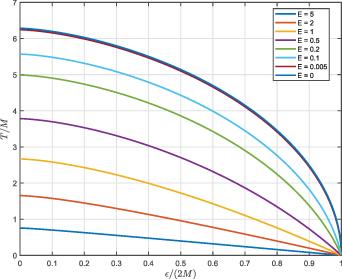
Figure 2. The black hole-white hole transfer time comparison for different ϵ-Schwarzschild spacetimes. |
Our analysis indicates that the transfer time of ϵ-Schwarzschild is the same order of the mass of the black hole. For stellar massive black holes, the transfer time is about a microsecond. For super-massive black holes like the one locating at the center of our galaxy, the transfer time is about a second. If we take the ϵ correction as the quantum effect, this quantum effect makes the black hole-white hole transition faster. This ϵ plays a role as a quantum scale. If such a quantum scale exists, the black hole must be larger than $r_\mathrm{H} \gt \epsilon$ where $r_\mathrm{H}$ is the size of the horizon.
In order to check the quantum behavior of the ϵ-Schwarzschild model recovering the classical limit, we compare the black hole-white hole transfer time comparison for different ϵ-Schwarzschild spacetimes to 0-Schwarzschild spacetimes in figure 3. From this figure we can see that the transferring object with smaller energy is easier to explore the quantum effect. Anyhow, if only the black hole mass $M\gt 3\epsilon$, the quantum effect is ignorable.
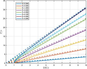
Figure 3. Comparison of the black hole-white hole transfer time comparison for different ϵ-Schwarzschild spacetimes to 0-Schwarzschild spacetimes. |
The ϵ-Schwarzschild model represents a simplified regularization scheme. More sophisticated approaches, such as the Simpson-Visser model [11], can be viewed as refinements that implement similar regularization through minimal length parameters while maintaining better physical properties. The Simpson-Visser metric introduces a minimal length scale a
$\begin{align} \mathrm{d}s^2 & = -\left(1 - \frac{2M}{\sqrt{r^2 + a^2}}\right) \mathrm{d}t^2 + \left(1 - \frac{2M}{\sqrt{r^2 + a^2}}\right)^{-1} \mathrm{d}r^2\nonumber\\ & \quad + \left(r^2 + a^2\right) \mathrm{d}\Omega^2.\end{align}$
The black hole and white hole horizons are located at
$align$
The transfer time can be calculated as $equation$
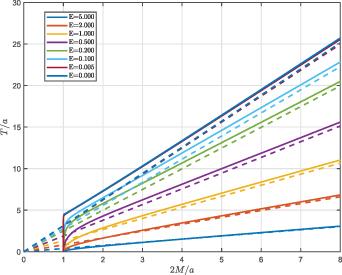
We plot this transfer time in figures 4 and 5. This quantum effect reshapes just the black hole-white hole transition without essential difference compared to ϵ-Schwarzschild spacetimes. Especially, when $M\gt 3a$, the quantum effect is ignorable. On the extremal quantum side $M = a/2$, the transfer time is always 0 independent of the energy E.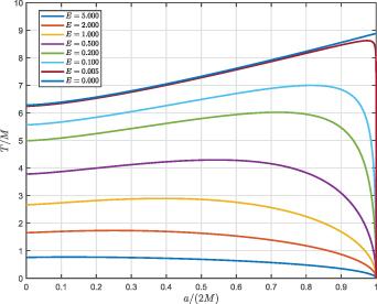
4. Transfer time of RN type spacetimes
The authors of [5] have deduced a Swiss cheese model of a black hole within the loop quantum gravity theory 13 ), there are no black holes or white holes at all.
$\begin{align} \mathrm{d}s^2 &= -\left(1-\frac{2M}{r}+\alpha\frac{M^2}{r^4}\right)\mathrm{d}t^2\nonumber\\ & \quad +\left(1-\frac{2M}{r}+\alpha\frac{M^2}{r^4}\right)^{-1}\mathrm{d}r^2+r^2\mathrm{d}\Omega^2,\end{align}$
$align$
where $l_\mathrm{p}$ is the Planck length and γ is the Barbero-Immirzi parameter of the loop quantum gravity. The black hole and white hole horizon are located at $align$
where β is the solution of the algebra equation $align$
in the range $1/2 \lt \beta\lt 1$. The above relations indicate that there is a minimal black hole mass $align$
When the parameter $M\lt M_\textrm{min}$ in (For the time-like geodesic along the radial direction we have
$align$
Corresponding to the transfer time problem, we are now interested in the time-like geodesic results in r which decrease from $r_+$ to $r_\textrm{min}$ and then increase to $r_+$. This turning point $r_\textrm{min}$ corresponds to the solution of $align$
Then the black hole-white hole transfer time can be expressed as $\begin{align} T& = 2\int_{r_\textrm{min}}^{r_+}\frac{1}{\sqrt{E^2-1+\frac{2M}{r}-\alpha\frac{M^2}{r^4}}}\mathrm{d}r\nonumber\\ & = 2\int_{r_\textrm{min}}^{r_+}\frac{1}{\sqrt{E^2-1+\frac{2M}{r}-\frac{27}{16}\frac{M_\textrm{min}^2M^2}{r^4}}}\mathrm{d}r.\end{align}$
When $M_\textrm{min}$ goes to zero, the 0-Schwarzschild result is recovered. When $M_\textrm{min}$ increases, the quantum effect becomes stronger. If $M_\textrm{min} = M$, the inner horizon coincides with the outer horizon. But we still have the black hole-white hole transition. In contrast, if $M_\textrm{min}\gt M$ the black hole horizon disappears. There is no black hole-white hole transition any more. Consequently the transfer time vanishes. This means the transfer time as a function of $M_\textrm{min}$ is not continuous at $M_\textrm{min} = M$.
We plot the transfer time T respective to $M_\textrm{min}/M\in(0,1)$ in figure 6 for several given E. From the plot we can see an interesting feature of the function T respective to energy E and the spacetime parameter $M_\textrm{min}/M$
$align$
$align$
but very outstandingly $\begin{align} \frac{3\sqrt{2}\pi}{4}M &= \lim_{E\rightarrow0}T\left(E,M_\textrm{min} = M\right)\neq \lim_{M_\textrm{min}\rightarrow M}T\left(E = 0,M_\textrm{min}\right)\nonumber\\ & = \frac{3\sqrt{2}\pi}{2}M.\end{align}$
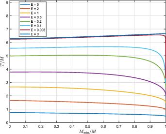
Figure 6. Similar to figure 2 but for the Swiss cheese model within loop quantum gravity. |
We find that the above T behavior is very similar to the one for RN spacetime. Corresponding to figure 6 we plot the transfer time T respective to $Q/M\in(0,1)$ in figure 7 for RN spacetime. Here Q is the electric charge of the spacetime. Corresponding to equations (21 )-(23 ), we have
$align$
$align$
$\begin{align} \pi M &= \lim_{E\rightarrow0}T\left(E,Q = M\right)\neq \lim_{Q\rightarrow M}T\left(E = 0,Q\right)\nonumber\\ & = 2\pi M.\end{align}$
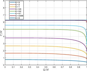
Figure 7. Similar to figure 2 but for Reissner-Nordstromöm spacetime. |
On the one hand, the RN type spacetimes admit special transfer time behavior for extremal cases $p/M = 1$ where p is the RN type quantum parameter. On the other hand, we can also see the transfer time behavior becomes more and more similar to that of 0-Schwarzschild spacetimes for larger black holes. We show such behavior in figure 8. We find that if only $M\gt 3p$, the 0-Schwarzschild spacetime can approximate the regular black holes very well.
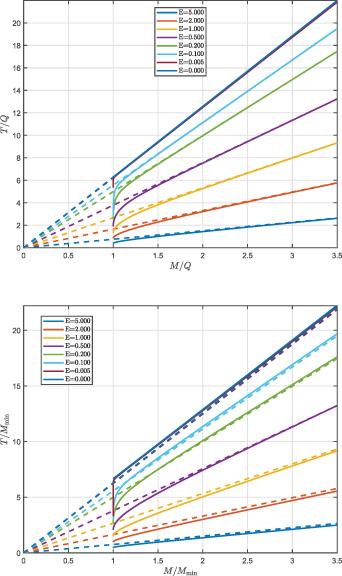
Figure 8. Similar to figure 3 but for RN type spacetimes. Top: the Reissner-Nordstromöm spacetimes. Bottom: the Swiss cheese model within loop quantum gravity. |
We would like to notice that the transfer time behavior similarity of the RN type regular black hole models only means the spacetime geometry admits some similarity to that of the RN black holes. This fact does not mean RN black holes contain any quantum effects.
5. Transfer time of Hayward type spacetimes
The Bianchi-Christodoulou-D'Ambrosio-Haggard-Rovelli (BCDHR) model [10] provides an alternative regularization inspired by loop quantum gravity
$align$
$align$
where l is a quantum parameter. When l = 0, $\begin{align} \mathrm{d}s^2& = -\frac{\xi^2-2M}{\xi^2}\mathrm{d}t^2+\frac{4\xi^4}{\xi^2-2M}\mathrm{d}\xi^2+\xi^4\mathrm{d}\Omega^2\nonumber\\ & = -\frac{\xi^2-2M}{\xi^2}\mathrm{d}t^2+\frac{\xi^2}{\xi^2-2M}\left(2\xi \mathrm{d}\xi\right)^2+\xi^4\mathrm{d}\Omega^2\nonumber\\ & = -\frac{\xi^2-2M}{\xi^2}\mathrm{d}t^2+\frac{\xi^2}{\xi^2-2M}\left(\mathrm{d}\xi^2\right)^2+\xi^4\mathrm{d}\Omega^2,\nonumber\\ r&\equiv\xi^2,\end{align}$
$align$
which recovers the Schwarzschild metric.The boundary of the regions containing trapping and anti-trapping surfaces correspond to the apparent horizon
$align$
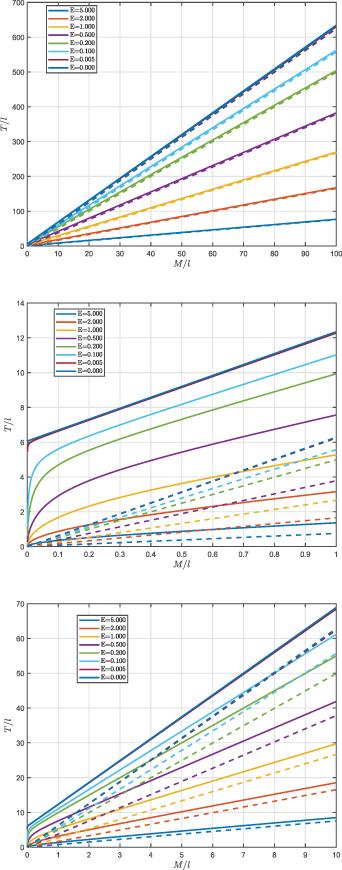
We accordingly take them as the boundary of black holes and white holes. The corresponding transfer time is $equation$
Unlike the above mentioned Schwarzschild type and RN type spacetimes, where horizons will disappear if the quantum parameter is too large, the horizons always exist in BCDHR spacetimes no matter how large the parameter l is. When $l \gg M$
$equation$
the transfer time approaches to infinite and scales as $T \propto \sqrt{l}$.We plot this transfer time in figures 9 and 10. From figure 9 we find that the quantum effect of the BCDHR model increases the transfer time which is different to the behavior in the above mentioned Schwarzschild type and RN type spacetimes. From the top panel of figure 10 we can see if the black hole mass is larger than several tens of quantum parameter l, the 0-Schwarzschild model can describe the transfer time behavior well. When $M\lt 10l$ the quantum behavior shows up. In the bottom panel of figure 10 we can see that the quantum effect becomes significant when M < l.


6. Discussion and conclusion
More and more observations including gravitational waves and black hole shadows indicate the existence of black holes in our Universe. Within the GR theory, Penrose and Hawking have proved the famous mathematical theorem of singularity which states that a singularity must appear inside of a black hole. This theorem indicates that the GR must fail near the extremely strong field region in a black hole. Although more and more observations indicate that GR is the best theory to describe gravity, people believe singularity is unphysical. Unfortunately, it is still unknown what kind of theories are correct when GR breaks down.
Based on the observation evidence that black holes should exist and the above mentioned belief that singularity should not appear, people have proposed many models to describe black holes without singularity. Such models are called regular black holes. One interesting and important question is which model is correct to describe the nature.
Most regular black hole models have white holes following the black hole. In the current paper we propose a concept of transfer time of black hole-white hole. We find in the current paper that there are three catalogs of behavior of the transfer time of black hole-white hole. These three catalogs admit qualitatively different behavior. Possibly some stars form when matter falls into the pre-black hole, so the life of such stars can reflect the transfer time of a black hole-white hole. In the near future, if we can use observations such as the life of a star to estimate the transfer time of a black hole-white hole, correct regular black hole models can be recognized accordingly. Based on these distinguished regular black hole models, we can understand the property of extremely strong gravity better.
Regarding the above mentioned stellar lifetime observation, there is a subtle point that needs to be highlighted. Let us firstly consider an analogous example. Person A observes person B. Person A finds that person B has white hair, consequently person A deduces that person B is about 60 years old. Such an estimation is irrelevant to person A's time. So person A can conclude that from the birth of person B to the time point that person B is observed, the proper time of person B has lasted 60 years. The stellar lifetimes observation is very similar. People can deduce the lifetime of a stellar based on the element status and other properties. In another world, we should not confuse the lifetime observation here with the proper time of the observer itself. Instead, the stellar lifetime should be related to the transfer time discussed in the current paper.
The current paper discussed the possible classification of regular black hole models. But we also need to be aware that the current paper only touches on regular black hole models which admit both black holes and white holes. There are indeed some regular black hole models which do not admit white holes. For example, the regular black holes with de Sitter core belong to this type. Such models do not fall into the discussion objects of the current work.