

1. Introduction
The theoretical description of Bose-Einstein condensates (BECs) is of fundamental importance for capturing their quantum nature [1, 2]. So far, the coherent-state-based Gross-Pitaevskii equation (GPE) [3, 4], along with the perturbative Bogoliubov excitations around ground states [5, 6], has achieved great success when describing the BECs of dilute atomic gases [2, 7]. The bosonic version of Hartree-Fock-Bogoliubov (HFB) formalism [5, 8-11], which provides a self-consistent treatment of the fluctuations, is a natural generalization of the GPE plus Bogoliubov theory. Although the HFB formalism can provide satisfactory results in both zero- and finite-temperature problems [7, 12-14], it fails to yield the gapless excitation spectrum [11, 15], which violates the Hugenholtz-Pines theorem [9]. By adopting a Gaussian-state ansatz (i.e., squeezed-coherent state for a bosonic gas), the Gaussian-state theory (GST) [16], which is equivalent to the HFB theory for the ground-state solutions, takes a completely different route to treat the quantum fluctuations. Specifically, when treating the fluctuation around a ground state, it also incorporates the fluctuations of the correlation functions, which successfully produces the gapless excitation spectrum [17-19]. Physically, the fluctuations of the correlation functions represent two-particle excitations.
As an application of GST to BECs, we considered the simplest scenario by studying the ground states and excitations of a trapped atomic gas with contact interaction [18]. Interestingly, it was found that the ground state of a condensate with weakly attractive interaction becomes a single-mode squeezed vacuum state (SVS), as opposed to the coherent state (CS) under repulsive interaction. Other systems that fit GST studies well are the self-bound quantum droplets in both dipolar and two-component condensates [20-26]. These systems have been widely investigated using the extended GPE [27-30], which is a generalized GPE that includes the contribution of the fluctuation through the perturbative Lee-Huang-Yang correction [31]. Along this direction, we explored the quantum phases of both dipolar and binary droplets in the presence of three-body repulsion [32, 33]. Generally, in the low-density regime, where the interaction is purely attractive, the condensate belongs to the SVS phase, whereas in the high-density regime, where the three-body repulsion dominates, the condensate is in the CS phase. Moreover, for the parameter regime between the SVS and CS phases, the system falls into a single-mode squeezed-coherent state (SCS). Finally, we also studied the collapse dynamics of a trapped single-component condensate using the Gaussian state theory (GST) for mixed states [33], which revealed a distinct type of collapse assisted by fluctuations through amplifying the attractive interaction between atoms.
Technically, to obtain the ground state, one needs to simultaneously evolve, in imaginary time, the normal and anomalous correlation functions of the condensate wave function. This poses a serious challenge for numerical calculations, as it requires tremendous computing resources and even becomes computationally intractable for three-dimensional systems without sufficient symmetries. To reduce the demand for computing resources, we note that a Gaussian state can always be factorized into a multimode coherent-squeezed state [32, 33]. Since, in practice, only a few squeezed modes are highly occupied, we may approximate the Gaussian state by one that involves the coherent mode and these highly occupied squeezed modes. In the present work, we develop the effective Gaussian-state theory (EGST) by deriving the imaginary-time evolution equations for the squeezed modes and the occupation numbers. We then calibrate these effective equations in a Bose gas of self-bound dipolar droplets. We show that the EGST results converge to those obtained via the full GST when the number of squeezed modes included in the calculation is sufficiently large. Particularly, for the SVS and SCS phases of dipolar droplets in which the number of notably occupied squeezed modes is small, the EGST approach has a substantial advantage over the full GST.
The rest of this paper is organized as follows. In section 2, we briefly recall GST. In section 3 , we present an alternative approach to factorize the Gaussian state into the form of a multimode squeezed-coherent state. We derive, in section 4 , the imaginary-time evolution equations for the highly populated squeezed modes and the corresponding occupation numbers. These equations constitute the effective theory for GST, and their solution yields an approximate ground state very close to that obtained via the full GST. In section 5 , we validate the effective Gaussian-state approach by revisiting the system of dipolar droplets. We show that the effective theory improves the efficiency of numerical calculations, in particular when the number of squeezed modes involved in the ground state is small. Finally, we conclude in section 6 .
2. Gaussian state theory
We begin by briefly reviewing GST for bosons [34]. For a many-body quantum system, a pure Gaussian state takes the form 1 ), we have introduced shorthand notations, in which the products in the exponents denote matrix products in the Nambu space and integration in the coordinate space, i.e.,
$\begin{eqnarray}\begin{array}{rc}| {\rm{GS}}\rangle & ={\widehat{{\mathscr{U}}}}_{{\rm{GS}}}| 0\rangle ={{\rm{e}}}^{{\rm{i}}\theta }{{\rm{e}}}^{{\widehat{{\rm{\Psi }}}}^{\dagger }{{\rm{\Sigma }}}_{z}{\rm{\Phi }}}{{\rm{e}}}^{\frac{{\rm{i}}}{2}{\widehat{{\rm{\Psi }}}}^{\dagger }{\rm{\Xi }}\widehat{{\rm{\Psi }}}}| 0\rangle ,\end{array}\end{eqnarray}$
where ${\widehat{{\mathscr{U}}}}_{{\rm{GS}}}$ is a unitary operator, θ is a global phase, $\widehat{{\rm{\Psi }}}({\boldsymbol{r}})=\left(\begin{array}{c}\widehat{\psi }({\boldsymbol{r}})\\ {\widehat{\psi }}^{\dagger }({\boldsymbol{r}})\end{array}\right)$ is the bosonic field operator satisfying the commutation relation $[\widehat{{\rm{\Psi }}}({\boldsymbol{r}}),{\widehat{{\rm{\Psi }}}}^{\dagger }({{\boldsymbol{r}}}^{{\prime} })]={{\rm{\Sigma }}}_{z}({\boldsymbol{r}},{{\boldsymbol{r}}}^{{\prime} })$ [$\equiv {\sigma }_{z}\otimes \delta ({\boldsymbol{r}}-{{\boldsymbol{r}}}^{{\prime} })$ with σz being the Pauli matrix], and ${\rm{\Phi }}({\boldsymbol{r}})=\left(\begin{array}{c}\phi ({\boldsymbol{r}})\\ {\phi }^{* }({\boldsymbol{r}})\end{array}\right)$ and ${\rm{\Xi }}({\boldsymbol{r}},{{\boldsymbol{r}}}^{{\prime} })=\left(\begin{array}{cc}{\xi }_{11}({\boldsymbol{r}},{{\boldsymbol{r}}}^{{\prime} }) & {\xi }_{12}({\boldsymbol{r}},{{\boldsymbol{r}}}^{{\prime} })\\ {\xi }_{12}^{\dagger }({\boldsymbol{r}},{{\boldsymbol{r}}}^{{\prime} }) & {\xi }_{11}^{{\rm{T}}}({\boldsymbol{r}},{{\boldsymbol{r}}}^{{\prime} })\end{array}\right)$ are variational parameters. Particularly, the unitarity of ${\widehat{{\mathscr{U}}}}_{{\rm{GS}}}$ requires that ξ11 and ξ12 are, respectively, Hermitian and symmetric matrices with respect to the indices r and ${{\boldsymbol{r}}}^{{\prime} }$, i.e., ${\xi }_{11}^{{\rm{T}}}({\boldsymbol{r}},{{\boldsymbol{r}}}^{{\prime} })={\xi }_{11}^{* }({\boldsymbol{r}},{{\boldsymbol{r}}}^{{\prime} })$ and ${\xi }_{12}^{\dagger }({\boldsymbol{r}},{{\boldsymbol{r}}}^{{\prime} })={\xi }_{12}^{* }({\boldsymbol{r}},{{\boldsymbol{r}}}^{{\prime} })$. In equation ($\begin{eqnarray*}\begin{array}{rcl}{\widehat{{\rm{\Psi }}}}^{\dagger }{{\rm{\Sigma }}}_{z}{\rm{\Phi }} & \equiv & \displaystyle \int {\rm{d}}{\boldsymbol{r}}{\rm{d}}{{\boldsymbol{r}}}^{{\prime} }\left(\begin{array}{cc}{\widehat{\psi }}^{\dagger }({\boldsymbol{r}}) & \widehat{\psi }({\boldsymbol{r}})\end{array}\right)\\ & & \times \left(\begin{array}{cc}\delta ({\boldsymbol{r}}-{{\boldsymbol{r}}}^{{\prime} }) & 0\\ 0 & -\delta ({\boldsymbol{r}}-{{\boldsymbol{r}}}^{{\prime} })\end{array}\right)\left(\begin{array}{c}\phi ({{\boldsymbol{r}}}^{{\prime} })\\ {\phi }^{* }({{\boldsymbol{r}}}^{{\prime} })\end{array}\right),\\ {\widehat{{\rm{\Psi }}}}^{\dagger }{\rm{\Xi }}\widehat{{\rm{\Psi }}} & \equiv & \displaystyle \int {\rm{d}}{\boldsymbol{r}}{\rm{d}}{{\boldsymbol{r}}}^{{\prime} }\left(\begin{array}{cc}{\widehat{\psi }}^{\dagger }({\boldsymbol{r}}) & \widehat{\psi }({\boldsymbol{r}})\end{array}\right)\\ & & \times \left(\begin{array}{cc}{\xi }_{11}({\boldsymbol{r}},{{\boldsymbol{r}}}^{{\prime} }) & {\xi }_{12}({\boldsymbol{r}},{{\boldsymbol{r}}}^{{\prime} })\\ {\xi }_{12}^{\dagger }({\boldsymbol{r}},{{\boldsymbol{r}}}^{{\prime} }) & {\xi }_{11}^{{\rm{T}}}({\boldsymbol{r}},{{\boldsymbol{r}}}^{{\prime} })\end{array}\right)\left(\begin{array}{c}\widehat{\psi }({{\boldsymbol{r}}}^{{\prime} })\\ {\widehat{\psi }}^{\dagger }({{\boldsymbol{r}}}^{{\prime} })\end{array}\right).\end{array}\end{eqnarray*}$
For convenience, we introduce two unitary operators, i.e., the displacement operator $\widehat{{\mathscr{D}}}({\rm{\Phi }})\equiv {{\rm{e}}}^{{\widehat{{\rm{\Psi }}}}^{\dagger }{{\rm{\Sigma }}}_{z}{\rm{\Phi }}}$ and the squeezing operator $\widehat{{\mathscr{S}}}(\xi )\equiv {{\rm{e}}}^{\frac{{\rm{i}}}{2}{\widehat{{\rm{\Psi }}}}^{\dagger }{\rm{\Xi }}\widehat{{\rm{\Psi }}}}$. One can easily verify that 5 ).
$\begin{eqnarray}\begin{array}{rc}{\widehat{{\mathscr{D}}}}^{\dagger }({\rm{\Phi }})\widehat{{\rm{\Psi }}}\widehat{{\mathscr{D}}}({\rm{\Phi }}) & =\widehat{{\rm{\Psi }}}+{\rm{\Phi }},\end{array}\end{eqnarray}$
$\begin{eqnarray}\begin{array}{rc}{\widehat{{\mathscr{S}}}}^{\dagger }(\xi )\widehat{{\rm{\Psi }}}\widehat{{\mathscr{S}}}(\xi ) & ={\mathbb{S}}(\xi )\widehat{{\rm{\Psi }}},\end{array}\end{eqnarray}$
where ${\rm{\Phi }}=\langle \widehat{{\rm{\Psi }}}\rangle $ and ${\mathbb{S}}(\xi )={{\rm{e}}}^{{\rm{i}}{{\rm{\Sigma }}}_{z}{\rm{\Xi }}}$. It is convenient to rewrite ${\mathbb{S}}(\xi )$ as a matrix of the form $\begin{eqnarray}\begin{array}{r}{\mathbb{S}}(\xi )=\left(\begin{array}{cc}{{\mathbb{S}}}_{11}({\boldsymbol{r}},{{\boldsymbol{r}}}^{{\prime} }) & {{\mathbb{S}}}_{12}({\boldsymbol{r}},{{\boldsymbol{r}}}^{{\prime} })\\ {{\mathbb{S}}}_{21}({\boldsymbol{r}},{{\boldsymbol{r}}}^{{\prime} }) & {{\mathbb{S}}}_{22}({\boldsymbol{r}},{{\boldsymbol{r}}}^{{\prime} })\end{array}\right),\end{array}\end{eqnarray}$
where ${{\mathbb{S}}}_{21}={{\mathbb{S}}}_{12}^{* }$ and ${{\mathbb{S}}}_{22}={{\mathbb{S}}}_{11}^{* }$. Moreover, from the bosonic commutation relation of $\widehat{{\rm{\Psi }}}$, we have ${\widehat{{\mathscr{S}}}}^{\dagger }(\xi )[\widehat{{\rm{\Psi }}},{\widehat{{\rm{\Psi }}}}^{\dagger }]\widehat{{\mathscr{S}}}(\xi )={{\rm{\Sigma }}}_{z}$, and therefore $\begin{eqnarray}\begin{array}{rc}{\mathbb{S}}{{\rm{\Sigma }}}_{z}{{\mathbb{S}}}^{\dagger } & ={{\rm{\Sigma }}}_{z},\end{array}\end{eqnarray}$
which indicates that ${\mathbb{S}}$ is symplectic and represents a canonical transformation. Alternatively, using the Taylor expansion of ${\mathbb{S}}$, it can be shown that $\begin{eqnarray}\begin{array}{rc}{{\rm{\Sigma }}}_{z}{{\mathbb{S}}}^{\dagger }{{\rm{\Sigma }}}_{z} & ={{\mathbb{S}}}^{-1},\end{array}\end{eqnarray}$
which also gives rise to equation (It is important to note that there is a gauge redundancy in the variational wave function, as different ξ's may lead to the same Gaussian state. In fact, any unitary operator $\widehat{{\mathscr{V}}}$ satisfying $\widehat{{\mathscr{V}}}| 0\rangle =| 0\rangle $ leaves the Gaussian state unchanged, since ${\widehat{{\mathscr{U}}}}_{{\rm{GS}}}\widehat{{\mathscr{V}}}| 0\rangle ={\widehat{{\mathscr{U}}}}_{{\rm{GS}}}| 0\rangle $. Thus, ${\widehat{{\mathscr{U}}}}_{{\rm{GS}}}\widehat{{\mathscr{V}}}$ defines a new Gaussian-state operator. As a concrete example, we consider an operator $\widehat{{\mathscr{V}}}={{\rm{e}}}^{{\rm{i}}{\widehat{\psi }}^{\dagger }{\chi }_{11}\widehat{\psi }}$ with ${\chi }_{11}^{\dagger }={\chi }_{11}$, which, in the Nambu space, can be rewritten as $\widehat{{\mathscr{V}}}={{\rm{e}}}^{\frac{{\rm{i}}}{2}{\widehat{{\rm{\Psi }}}}^{\dagger }{{\rm{\Xi }}}_{0}\widehat{{\rm{\Psi }}}}$, where ${{\rm{\Xi }}}_{0}=\left(\begin{array}{cc}{\chi }_{11} & 0\\ 0 & {\chi }_{11}^{* }\end{array}\right)$. Since there exists ${{\rm{\Xi }}}^{{\prime} }$ such that ${{\rm{e}}}^{\frac{{\rm{i}}}{2}{\widehat{{\rm{\Psi }}}}^{\dagger }{{\rm{\Xi }}}^{{\prime} }\widehat{{\rm{\Psi }}}}={{\rm{e}}}^{\frac{{\rm{i}}}{2}{\widehat{{\rm{\Psi }}}}^{\dagger }{\rm{\Xi }}\widehat{{\rm{\Psi }}}}{{\rm{e}}}^{\frac{{\rm{i}}}{2}{\widehat{{\rm{\Psi }}}}^{\dagger }{{\rm{\Xi }}}_{0}\widehat{{\rm{\Psi }}}}$, the redundancy in Ξ is then confirmed.
To remove this redundancy, we replace the variational parameter Ξ by the covariance matrix ${\rm{\Gamma }}\equiv \langle \{\delta \widehat{{\rm{\Psi }}},\delta {\widehat{{\rm{\Psi }}}}^{\dagger }\}\rangle $, where $\delta \widehat{{\rm{\Psi }}}\equiv \widehat{{\rm{\Psi }}}-{\rm{\Phi }}$ is the fluctuation field and {, } represents the anti-commutator. Γ and Ξ are related as follows:
$\begin{eqnarray}\begin{array}{rcl}{\rm{\Gamma }} & = & \langle {\rm{GS}}| \left\{\delta \widehat{{\rm{\Psi }}},\delta {\widehat{{\rm{\Psi }}}}^{\dagger }\right\}| {\rm{GS}}\rangle \\ & = & \langle 0| {\widehat{{\mathscr{S}}}}^{\dagger }{\widehat{{\mathscr{D}}}}^{\dagger }\left\{\delta \widehat{{\rm{\Psi }}},\delta {\widehat{{\rm{\Psi }}}}^{\dagger }\right\}\widehat{{\mathscr{D}}}\widehat{{\mathscr{S}}}| 0\rangle \\ & = & {\mathbb{S}}{{\mathbb{S}}}^{\dagger }.\end{array}\end{eqnarray}$
The matrix ${\mathbb{S}}$ has a unitary freedom, as Γ remains unchanged under the transformation ${\mathbb{S}}\to {\mathbb{S}}\left(\begin{array}{cc}{ \mathcal W } & 0\\ 0 & {{ \mathcal W }}^{* }\end{array}\right)$, with ${ \mathcal W }$ being an arbitrary unitary matrix. This unitary freedom is associated with the redundancy of Ξ, which, as shown below, can be removed by requiring that Ξ only contains off-diagonal blocks in Nambu space. It is also worth noting that Γ satisfies $\begin{eqnarray}\begin{array}{rcl}{\rm{\Gamma }}{{\rm{\Sigma }}}_{z}{\rm{\Gamma }} & = & {\mathbb{S}}{{\mathbb{S}}}^{\dagger }{{\rm{\Sigma }}}_{z}{\mathbb{S}}{{\mathbb{S}}}^{\dagger }\\ & = & {\mathbb{S}}{{\rm{\Sigma }}}_{z}{{\rm{\Sigma }}}_{z}{{\mathbb{S}}}^{\dagger }{{\rm{\Sigma }}}_{z}{\mathbb{S}}{{\mathbb{S}}}^{\dagger }\\ & = & {\mathbb{S}}{{\rm{\Sigma }}}_{z}{{\mathbb{S}}}^{-1}{\mathbb{S}}{{\mathbb{S}}}^{\dagger }\\ & = & {{\rm{\Sigma }}}_{z}.\end{array}\end{eqnarray}$
For the ground state of a system described by Hamiltonian $\widehat{H}$, the Gaussian state wave function can be determined by minimizing the energy ${E}_{0}=\langle {\rm{GS}}| \widehat{H}| {\rm{GS}}\rangle $ with respect to Φ and Γ. This is equivalent to evolve a trial Gaussian state ∣GS⟩ in imaginary time τ until it converges. As shown in [34], the imaginary-time evolution of a wave function is governed by the equation 5 .
$\begin{eqnarray}\begin{array}{r}{\partial }_{\tau }| {\rm{GS}}\rangle =-({\widehat{H}}_{{\rm{MF}}}-{E}_{0})| {\rm{GS}}\rangle .\end{array}\end{eqnarray}$
Here ${\widehat{H}}_{{\rm{MF}}}$ is the mean-field Hamiltonian, which is obtained by replacing $\widehat{\psi }$ in the Hamiltonian $\widehat{H}$ with $\phi +\delta \widehat{\psi }$, applying Wick's theorem with respect to the Gaussian state, and retaining terms up to the quadratic order in $\delta \widehat{\psi }$. Eventually, ${\widehat{H}}_{{\rm{MF}}}$ can be generally expressed as $\begin{eqnarray}{\widehat{H}}_{{\rm{MF}}}={E}_{0}+\delta {\widehat{{\rm{\Psi }}}}^{\dagger }{\rm{\Upsilon }}+\frac{1}{2}:\delta {\widehat{{\rm{\Psi }}}}^{\dagger }{\mathbb{H}}\delta \widehat{{\rm{\Psi }}}{:}_{{\rm{GS}}},\end{eqnarray}$
where ϒ(r) = $\left(\begin{array}{c}\eta ({\boldsymbol{r}})\\ {\eta }^{* }({\boldsymbol{r}})\end{array}\right)$, ${\mathbb{H}}({\boldsymbol{r}},{{\boldsymbol{r}}}^{{\prime} })=\left(\begin{array}{cc}{ \mathcal E }({\boldsymbol{r}},{{\boldsymbol{r}}}^{{\prime} }) & {\rm{\Delta }}({\boldsymbol{r}},{{\boldsymbol{r}}}^{{\prime} })\\ {{\rm{\Delta }}}^{\dagger }({\boldsymbol{r}},{{\boldsymbol{r}}}^{{\prime} }) & {{ \mathcal E }}^{{\rm{T}}}({\boldsymbol{r}},{{\boldsymbol{r}}}^{{\prime} })\end{array}\right)$, and $:\widehat{O}{:}_{{\rm{GS}}}$ denotes the normal ordered operator with respect to the Gaussian state. Clearly, to find the explicit expressions for η, ${ \mathcal E }$, and Δ, one has to specify the Hamiltonian $\widehat{H}$ as demonstrated in section To proceed further, we derive, from equation (9 ), the imaginary-time equations of motion (ITEOM) for the variational parameters Φ and Γ. For this purpose, we first evaluate the left-hand side of equation (9 ) and find 9 ) reduces to 11 ) and (12 ), only those proportional to ${\widehat{\psi }}^{\dagger }$ and ${\widehat{\psi }}^{\dagger }{\widehat{\psi }}^{\dagger }$ give rise to nonzero results after acting on the vacuum state. Therefore, we can find the ITEOM for Φ and Γ by separately matching the coefficients of the terms ${\widehat{\psi }}^{\dagger }$ and ${\widehat{\psi }}^{\dagger }{\widehat{\psi }}^{\dagger }$.
$\begin{eqnarray}\begin{array}{r}{\partial }_{\tau }| {\rm{GS}}\rangle ={\widehat{{\mathscr{U}}}}_{{\rm{GS}}}\left[{\widehat{{\rm{\Psi }}}}^{\dagger }{{\mathbb{S}}}^{\dagger }{{\rm{\Sigma }}}_{z}{\partial }_{\tau }{\rm{\Psi }}+\frac{1}{2}:{\widehat{{\rm{\Psi }}}}^{\dagger }{{\mathbb{S}}}^{\dagger }{{\rm{\Sigma }}}_{z}({\partial }_{\tau }{\mathbb{S}})\widehat{{\rm{\Psi }}}{:}_{0}\right]| 0\rangle ,\end{array}\end{eqnarray}$
where $:\widehat{O}{:}_{0}$ denotes the normal ordered operator with respect to the vacuum state ∣0⟩. After some straightforward calculations, the right-hand side of equation ( $\begin{eqnarray}-({\widehat{H}}_{{\rm{MF}}}-{E}_{0})| {\rm{GS}}\rangle =-{\widehat{{\mathscr{U}}}}_{{\rm{GS}}}\left[{\widehat{{\rm{\Psi }}}}^{\dagger }{{\mathbb{S}}}^{\dagger }{\rm{\Upsilon }}+\frac{1}{2}:{\widehat{{\rm{\Psi }}}}^{\dagger }{{\mathbb{S}}}^{\dagger }{\mathbb{H}}{\mathbb{S}}\widehat{{\rm{\Psi }}}{:}_{0}\right]| 0\rangle .\end{eqnarray}$
For terms on the right-hand side of equations (For the ${\widehat{\psi }}^{\dagger }$ term, we have 13 ). Making use of equation (4 ), we obtain 13 ), immediately lead to 13 ) and (15 ), combining with (6 ), then give rise to
$\begin{eqnarray}\begin{array}{r}{\left({{\mathbb{S}}}^{\dagger }{{\rm{\Sigma }}}_{z}{\partial }_{\tau }{\rm{\Phi }}\right)}_{1}=-{\left({{\mathbb{S}}}^{\dagger }{\rm{\Upsilon }}\right)}_{1},\end{array}\end{eqnarray}$
where the subscript '1' ('2') denotes the upper (lower) vector in Nambu space. To establish the relation between the full-sized vectors, we consider the lower halves of the vectors in equation ( $\begin{eqnarray}\begin{array}{rc} & {\left({{\mathbb{S}}}^{\dagger }{\rm{\Upsilon }}\right)}_{2}={\left({{\mathbb{S}}}^{\dagger }{\rm{\Upsilon }}\right)}_{1}^{* }\\ & \,\rm{and}\,\quad {\left({{\mathbb{S}}}^{\dagger }{{\rm{\Sigma }}}_{z}{\partial }_{\tau }{\rm{\Phi }}\right)}_{2}=-{\left({{\mathbb{S}}}^{\dagger }{{\rm{\Sigma }}}_{z}{\partial }_{\tau }{\rm{\Phi }}\right)}_{1}^{* },\end{array}\end{eqnarray}$
which, by combining with equation ( $\begin{eqnarray}\begin{array}{rcl}{\left({{\mathbb{S}}}^{\dagger }{{\rm{\Sigma }}}_{z}{\partial }_{\tau }{\rm{\Phi }}\right)}_{2} & = & -{\left({{\mathbb{S}}}^{\dagger }{{\rm{\Sigma }}}_{z}{\partial }_{\tau }{\rm{\Phi }}\right)}_{1}^{* }={\left({{\mathbb{S}}}^{\dagger }{\rm{\Upsilon }}\right)}_{1}^{* }\\ & = & {\left({{\mathbb{S}}}^{\dagger }{\rm{\Upsilon }}\right)}_{2}.\end{array}\end{eqnarray}$
Equations ( $\begin{eqnarray}\begin{array}{r}{\partial }_{\tau }{\rm{\Phi }}=-{\rm{\Gamma }}{\rm{\Upsilon }}.\end{array}\end{eqnarray}$
For EOM of Γ, we match the ${\widehat{\psi }}^{\dagger }{\widehat{\psi }}^{\dagger }$ terms in equations (11 ) and (12 ), which gives rise to 5 ), ${{\mathbb{S}}}^{\dagger }{{\rm{\Sigma }}}_{z}{\partial }_{\tau }{\mathbb{S}}$ is anti-Hermitian, which further yields 19 ) by Σz from the left and by ${{\mathbb{S}}}^{\dagger }$ from the right, we obtain 7 ), eventually leads to 16 ) and (21 ) constitute the ITEOM for the Gaussian states [34].
$\begin{eqnarray}\begin{array}{r}{\left({{\mathbb{S}}}^{\dagger }{{\rm{\Sigma }}}_{z}{\partial }_{\tau }{\mathbb{S}}\right)}_{12}=-{\left({{\mathbb{S}}}^{\dagger }{\mathbb{H}}{\mathbb{S}}\right)}_{12},\end{array}\end{eqnarray}$
where the subscript 'ij' denotes the (i, j) block in the Nambu space. Using the result of equation ( $\begin{eqnarray}\begin{array}{r}{\left({{\mathbb{S}}}^{\dagger }{{\rm{\Sigma }}}_{z}{\partial }_{\tau }{\mathbb{S}}\right)}_{21}=-{\left({{\mathbb{S}}}^{\dagger }{{\rm{\Sigma }}}_{z}{\partial }_{\tau }{\mathbb{S}}\right)}_{12}^{\dagger }={\left({{\mathbb{S}}}^{\dagger }{\mathbb{H}}{\mathbb{S}}\right)}_{21}.\end{array}\end{eqnarray}$
Then for the full matrix in Nambu space, we have $\begin{eqnarray}\begin{array}{rc}{{\mathbb{S}}}^{\dagger }{{\rm{\Sigma }}}_{z}{\partial }_{\tau }{\mathbb{S}} & =-\frac{1}{2}\left({{\rm{\Sigma }}}_{z}{{\mathbb{S}}}^{\dagger }{\mathbb{H}}{\mathbb{S}}-{{\mathbb{S}}}^{\dagger }{\mathbb{H}}{\mathbb{S}}{{\rm{\Sigma }}}_{z}\right)+{\mathbb{Q}},\end{array}\end{eqnarray}$
where, since the first term on the right-hand side only contains the off-diagonal blocks of ${{\mathbb{S}}}^{\dagger }{{\rm{\Sigma }}}_{z}{\partial }_{\tau }{\mathbb{S}}$, ${\mathbb{Q}}$ is the block diagonal matrix accounting for the diagonal blocks. As a result, ${\mathbb{Q}}$ is also an anti-Hermitian matrix. Now, multiplying equation ( $\begin{eqnarray}\begin{array}{rc}\left({\partial }_{\tau }{\mathbb{S}}\right){{\mathbb{S}}}^{\dagger } & =-\frac{1}{2}\left({\rm{\Gamma }}{\mathbb{H}}{\rm{\Gamma }}-{{\rm{\Sigma }}}_{z}{\mathbb{H}}{{\rm{\Sigma }}}_{z}\right)+{\mathbb{S}}{{\rm{\Sigma }}}_{z}{\mathbb{Q}}{{\mathbb{S}}}^{\dagger },\end{array}\end{eqnarray}$
which, by making use of equation ( $\begin{eqnarray}\begin{array}{r}{\partial }_{\tau }{\rm{\Gamma }}={{\rm{\Sigma }}}_{z}{\mathbb{H}}{{\rm{\Sigma }}}_{z}-{\rm{\Gamma }}{\mathbb{H}}{\rm{\Gamma }}.\end{array}\end{eqnarray}$
Equations (Before moving to the next section, we would like to discuss the physical significance of the steady state, say ${{\mathbb{S}}}_{0}$, obtained from the ITEOM. When ${{\mathbb{S}}}_{0}$ is reached, we have ${\left({{\mathbb{S}}}_{0}^{\dagger }{{\rm{\Sigma }}}_{z}{\partial }_{\tau }{{\mathbb{S}}}_{0}\right)}_{12}=0$, which, according to equation (17 ), implies that the off-diagonal blocks of ${{\mathbb{S}}}_{0}^{\dagger }{\mathbb{H}}{{\mathbb{S}}}_{0}$ vanish. Furthermore, utilizing equation (4 ), it can be verified that both diagonal blocks of ${{\mathbb{S}}}_{0}^{\dagger }{\mathbb{H}}{{\mathbb{S}}}_{0}$ are Hermitian and satisfy ${\left({{\mathbb{S}}}_{0}^{\dagger }{\mathbb{H}}{{\mathbb{S}}}_{0}\right)}_{11}={\left({{\mathbb{S}}}_{0}^{\dagger }{\mathbb{H}}{{\mathbb{S}}}_{0}\right)}_{22}^{{\rm{T}}}$. Therefore, ${{\mathbb{S}}}_{0}^{\dagger }{\mathbb{H}}{{\mathbb{S}}}_{0}$ can always be diagonalized by a unitary matrix, say ${\overline{{\mathbb{V}}}}^{{\prime} }\equiv \left(\begin{array}{cc}{\overline{V}}^{{\prime} } & 0\\ 0 & {\overline{V}}^{{\prime} * }\end{array}\right)$, as 5 ), we obtain the Bogoliubov equation from equation (22 ), i.e., 22 ), we then have
$\begin{eqnarray}\begin{array}{r}{\overline{{\mathbb{V}}}}^{{\prime} \dagger }{{\mathbb{S}}}_{0}^{\dagger }{\mathbb{H}}{{\mathbb{S}}}_{0}{\overline{{\mathbb{V}}}}^{{\prime} }={\sigma }_{0}\displaystyle \otimes {\mathsf{\Omega }},\end{array}\end{eqnarray}$
where σ0 is the 2 × 2 unit matrix and ${\mathsf{\Omega }}$ is a diagonal matrix formed by the eigenenergies. Due to the unitary freedom of ${{\mathbb{S}}}_{0}$, we can always absorb ${\overline{{\mathbb{V}}}}^{{\prime} }$ into ${{\mathbb{S}}}_{0}$ to form ${{\mathbb{S}}}_{0}^{{\prime} }$ = ${{\mathbb{S}}}_{0}{\overline{{\mathbb{V}}}}^{{\prime} }$. Clearly, ${{\mathbb{S}}}_{0}^{{\prime} }$ gives rise to the same physics as ${{\mathbb{S}}}_{0}$ since ${{\mathbb{S}}}_{0}^{{\prime} }{{\mathbb{S}}}_{0}^{{\prime} \dagger }={{\mathbb{S}}}_{0}{{\mathbb{S}}}_{0}^{\dagger }={{\rm{\Gamma }}}_{0}$. The quadratic term of the mean-field Hamiltonian can now be diagonalized as $\begin{eqnarray}\begin{array}{rcl}:\delta {\widehat{{\rm{\Psi }}}}^{\dagger }{\mathbb{H}}\delta \widehat{{\rm{\Psi }}}{:}_{{\rm{GS}}} & = & :\delta {\widehat{{\rm{\Psi }}}}^{\dagger }{\left({{\mathbb{S}}}_{0}^{{\prime} }{{\mathbb{S}}}_{0}^{{\prime} -1}\right)}^{\dagger }{\mathbb{H}}{{\mathbb{S}}}_{0}^{{\prime} }{{\mathbb{S}}}_{0}^{{\prime} -1}\delta \widehat{{\rm{\Psi }}}{:}_{{\rm{GS}}}\\ & = & :{\left({{\mathbb{S}}}_{0}^{{\prime} -1}\delta \widehat{{\rm{\Psi }}}\right)}^{\dagger }{\sigma }_{0}\displaystyle \otimes {\mathsf{\Omega }}\left({{\mathbb{S}}}_{0}^{{\prime} -1}\delta \widehat{{\rm{\Psi }}}\right){:}_{{\rm{GS}}},\end{array}\end{eqnarray}$
from which we identify ${{\mathbb{S}}}_{0}^{{\prime} -1}\delta \widehat{{\rm{\Psi }}}$ as the Bogoliubov quasiparticle. Indeed, it can be verified that the Gaussian state ∣GS⟩ is the vacuum state of ${{\mathbb{S}}}_{0}^{{\prime} -1}\delta \widehat{{\rm{\Psi }}}$. Moreover, making use of equation ( $\begin{eqnarray}\begin{array}{r}{{\rm{\Sigma }}}_{z}{\mathbb{H}}{{\mathbb{S}}}_{0}^{{\prime} }={{\mathbb{S}}}_{0}^{{\prime} }({\sigma }_{z}\displaystyle \otimes {\mathsf{\Omega }}),\end{array}\end{eqnarray}$
which, in the conventional notation, takes the form $\begin{eqnarray}\begin{array}{r}\left(\begin{array}{cc}{ \mathcal E } & {\rm{\Delta }}\\ -{{\rm{\Delta }}}^{* } & -{{ \mathcal E }}^{* }\end{array}\right)\left(\begin{array}{cc}\overline{U} & {\overline{V}}^{* }\\ \overline{V} & {\overline{U}}^{* }\end{array}\right)=\left(\begin{array}{cc}\overline{U} & {\overline{V}}^{* }\\ \overline{V} & {\overline{U}}^{* }\end{array}\right)\left(\begin{array}{cc}{\mathsf{\Omega }} & 0\\ 0 & -{\mathsf{\Omega }}\end{array}\right).\end{array}\end{eqnarray}$
Here $\overline{U}=({u}_{1}({\boldsymbol{r}}),{u}_{2}({\boldsymbol{r}}),\cdots \,)$ and $\overline{V}=({v}_{1}({\boldsymbol{r}}),{v}_{2}({\boldsymbol{r}}),\cdots \,)$ are Bogoliubov modes, and ${\mathsf{\Omega }}$ are the energies of the Bogoliubov quasiparticle. Conversely, if ${\mathbb{H}}$ is diagonalized by ${{\mathbb{S}}}_{0}^{{\prime} }$ as equation ( $\begin{eqnarray}\begin{array}{rc}{{\rm{\Gamma }}}_{0}{\mathbb{H}}{{\rm{\Gamma }}}_{0} & ={{\mathbb{S}}}_{0}^{{\prime} }({\sigma }_{z}\displaystyle \otimes {\mathsf{\Omega }}){{\rm{\Sigma }}}_{z}{{\mathbb{S}}}_{0}^{{\prime} \dagger }={{\rm{\Sigma }}}_{z}{\mathbb{H}}{{\mathbb{S}}}_{0}^{{\prime} }{{\rm{\Sigma }}}_{z}{{\mathbb{S}}}_{0}^{{\prime} \dagger }\\ & ={{\rm{\Sigma }}}_{z}{\mathbb{H}}{{\rm{\Sigma }}}_{z},\end{array}\end{eqnarray}$
which implies that ∂τΓ0 = 0 and the Γ0 corresponds to a steady (ground) state.3. Mode decomposition
Previously, it was shown in [32] that a Gaussian state can be factorized into a multimode squeezed-coherent state. Here we present an alternative derivation for this factorization. For this purpose, we rewrite the covariance matrix as 28 ) into the relation equation (8 ), we find
$\begin{eqnarray}\begin{array}{r}{\rm{\Gamma }}=\left(\begin{array}{cc}{{\rm{\Gamma }}}_{11} & {{\rm{\Gamma }}}_{12}\\ {{\rm{\Gamma }}}_{12}^{\dagger } & {{\rm{\Gamma }}}_{11}^{{\rm{T}}}\end{array}\right)=2\left(\begin{array}{cc}{ \mathcal G } & { \mathcal F }\\ {{ \mathcal F }}^{* } & {{ \mathcal G }}^{* }\end{array}\right)+\left(\begin{array}{cc}{ \mathcal I } & 0\\ 0 & { \mathcal I }\end{array}\right),\end{array}\end{eqnarray}$
where ${ \mathcal G }({\boldsymbol{r}},{{\boldsymbol{r}}}^{{\prime} })=\langle \delta {\widehat{\psi }}^{\dagger }({{\boldsymbol{r}}}^{{\prime} })\delta \widehat{\psi }({\boldsymbol{r}})\rangle $ and ${ \mathcal F }({\boldsymbol{r}},{{\boldsymbol{r}}}^{{\prime} })=\langle \delta \widehat{\psi }({\boldsymbol{r}})\delta \widehat{\psi }({{\boldsymbol{r}}}^{{\prime} })\rangle $ are the normal and the anomalous correlation functions, respectively, and ${ \mathcal I }({\boldsymbol{r}},{{\boldsymbol{r}}}^{{\prime} })=\delta ({\boldsymbol{r}}-{{\boldsymbol{r}}}^{{\prime} })$ is the Dirac function. Apparently, ${ \mathcal G }({\boldsymbol{r}},{{\boldsymbol{r}}}^{{\prime} })$ is a positive-semidefinite matrix with respect to the indices r and ${{\boldsymbol{r}}}^{{\prime} }$ and ${ \mathcal F }({\boldsymbol{r}},{{\boldsymbol{r}}}^{{\prime} })$ is a complex symmetric one. As a result, we may diagonalize Γ11 using a unitary matrix $\overline{A}$, i.e., ${\overline{A}}^{\dagger }{{\rm{\Gamma }}}_{11}\overline{A}={{\mathsf{\Gamma }}}_{11}^{(d)}$ with ${{\mathsf{\Gamma }}}_{11}^{(d)}$ being a diagonal matrix with all elements being non-negative. We then rewrite Γ as $\begin{eqnarray}\begin{array}{r}{\rm{\Gamma }}=\left(\begin{array}{cc}\overline{A} & 0\\ 0 & {\overline{A}}^{* }\end{array}\right)\left(\begin{array}{cc}{{\mathsf{\Gamma }}}_{11}^{(d)} & {{\mathsf{\Gamma }}}_{12}^{{\prime} }\\ {({{\mathsf{\Gamma }}}_{12}^{{\prime} })}^{\dagger } & {{\mathsf{\Gamma }}}_{11}^{(d)}\end{array}\right)\left(\begin{array}{cc}{\overline{A}}^{\dagger } & 0\\ 0 & {\overline{A}}^{{\rm{T}}}\end{array}\right),\end{array}\end{eqnarray}$
where ${{\mathsf{\Gamma }}}_{12}^{{\prime} }={\overline{A}}^{\dagger }{{\rm{\Gamma }}}_{12}{\overline{A}}^{* }$ is also a complex symmetric matrix. After substituting equation ( $\begin{eqnarray}\begin{array}{r}{{\mathsf{\Gamma }}}_{11}^{(d)}{{\mathsf{\Gamma }}}_{12}^{{\prime} }-{{\mathsf{\Gamma }}}_{12}^{{\prime} }{{\mathsf{\Gamma }}}_{11}^{(d)}=0,\end{array}\end{eqnarray}$
which indicates that the matrix ${{\mathsf{\Gamma }}}_{12}^{{\prime} }$ can be diagonalized simultaneously in the non-degenerate subspace of ${{\mathsf{\Gamma }}}_{11}^{(d)}$. Even in the degenerate subspace of ${{\mathsf{\Gamma }}}_{11}^{(d)}$, the matrix ${{\mathsf{\Gamma }}}_{12}^{{\prime} }$ can be diagonalized by a unitary matrix ${\mathsf{B}}$ as ${{\mathsf{B}}}^{\dagger }{{\mathsf{\Gamma }}}_{12}^{{\prime} }{{\mathsf{B}}}^{* }={{\mathsf{\Gamma }}}_{12}^{(d)}$ according to the Autonne-Takagi diagonalization [35, 36], where ${{\mathsf{\Gamma }}}_{12}^{(d)}$ is a diagonal matrix. We note that the elements of ${{\mathsf{\Gamma }}}_{12}^{(d)}$ can always be chosen to be real and non-negative as the phase of a complex eigenvalue, say ${({{\mathsf{\Gamma }}}_{12}^{(d)})}_{j}=| {({{\mathsf{\Gamma }}}_{12}^{(d)})}_{j}| {{\rm{e}}}^{{\rm{i}}{\varphi }_{j}}$, can be absorbed into the corresponding mode function. With the redefined unitary matrix $W=\overline{A}{\mathsf{B}}$, Γ can be factorized as $\begin{eqnarray}\begin{array}{r}{\rm{\Gamma }}=\left(\begin{array}{cc}\overline{W} & 0\\ 0 & {\overline{W}}^{* }\end{array}\right)\left(\begin{array}{cc}{{\mathsf{\Gamma }}}_{11}^{(d)} & {{\mathsf{\Gamma }}}_{12}^{(d)}\\ {{\mathsf{\Gamma }}}_{12}^{(d)} & {{\mathsf{\Gamma }}}_{11}^{(d)}\end{array}\right)\left(\begin{array}{cc}{\overline{W}}^{\dagger } & 0\\ 0 & {\overline{W}}^{{\rm{T}}}\end{array}\right).\end{array}\end{eqnarray}$
Namely, Γ11 and Γ12 are now diagonalized simultaneously.To proceed further, we substitute equation (30 ) into equation (8 ) and find 34 ), it can be identified that ${N}_{s,j}\equiv {\sinh }^{2}{d}_{j}$ is the particle occupation number in the jth squeezed mode and Ns = ∑jNs,j is the total number of squeezed atoms. For convenience, we always assume that dj and, equivalently, Ns,j are sorted in descending order. We remark that, for the matrix $\overline{W}$, r and j should be regarded as row and column indices, respectively. Furthermore, the unitarity of $\overline{W}$ implies that
$\begin{eqnarray}\begin{array}{r}{[{{\mathsf{\Gamma }}}_{11}^{(d)}]}^{2}-{[{{\mathsf{\Gamma }}}_{12}^{(d)}]}^{2}={\mathsf{I}},\end{array}\end{eqnarray}$
which allows us to parameterize them as ${{\mathsf{\Gamma }}}_{11}^{(d)}=\cosh 2{\mathsf{D}}$ and ${{\mathsf{\Gamma }}}_{12}^{(d)}=\sinh 2{\mathsf{D}}$ with ${\mathsf{D}}$ being a diagonal matrix. Here ${\mathsf{I}}$ is the identity of the mode space, i.e., ${{\mathsf{I}}}_{ij}={\delta }_{ij}$. Then, under a suitable gauge, ${\mathbb{S}}$ takes the form $\begin{eqnarray}\begin{array}{rcl}{\mathbb{S}} & = & \left(\begin{array}{cc}\overline{W} & 0\\ 0 & {\overline{W}}^{* }\end{array}\right)\left(\begin{array}{cc}\cosh {\mathsf{D}} & \sinh {\mathsf{D}}\\ \sinh {\mathsf{D}} & \cosh {\mathsf{D}}\end{array}\right)\left(\begin{array}{cc}{\overline{W}}^{\dagger } & 0\\ 0 & {\overline{W}}^{{\rm{T}}}\end{array}\right)\\ & = & \left(\begin{array}{cc}\overline{W}\cosh {\mathsf{D}}{\overline{W}}^{\dagger } & \overline{W}\sinh {\mathsf{D}}{\overline{W}}^{{\rm{T}}}\\ {\overline{W}}^{* }\sinh {\mathsf{D}}{\overline{W}}^{\dagger } & {\overline{W}}^{* }\cosh {\mathsf{D}}{\overline{W}}^{{\rm{T}}}\end{array}\right)={{\rm{e}}}^{{\rm{i}}{{\rm{\Sigma }}}_{z}{\rm{\Xi }}},\end{array}\end{eqnarray}$
where ${\rm{\Xi }}=\left(\begin{array}{cc}0 & -{\rm{i}}\overline{W}{\mathsf{D}}{\overline{W}}^{{\rm{T}}}\\ {\rm{i}}{\overline{W}}^{* }{\mathsf{D}}{\overline{W}}^{\dagger } & 0\end{array}\right)$. Here the redundancy in Ξ has been removed by requiring that Ξ only contains off-diagonal blocks. Furthermore, the covariance matrix can now be parameterized as $\begin{eqnarray}\begin{array}{rcl}{\rm{\Gamma }} & = & 2\left(\begin{array}{cc}\overline{W}{\sinh }^{2}{\mathsf{D}}{\overline{W}}^{\dagger } & \overline{W}\sinh {\mathsf{D}}\cosh {\mathsf{D}}{\overline{W}}^{{\rm{T}}}\\ {\overline{W}}^{* }\sinh {\mathsf{D}}\cosh {\mathsf{D}}{\overline{W}}^{\dagger } & {\overline{W}}^{* }{\sinh }^{2}{\mathsf{D}}{\overline{W}}^{{\rm{T}}}\end{array}\right)\\ & & +\,\left(\begin{array}{cc}{ \mathcal I } & 0\\ 0 & { \mathcal I }\end{array}\right),\end{array}\end{eqnarray}$
from which we identify that $\begin{eqnarray}\begin{array}{r}{ \mathcal G }=\overline{W}{\sinh }^{2}{\mathsf{D}}{\overline{W}}^{\dagger }\,\rm{and}\,{ \mathcal F }=\overline{W}\sinh {\mathsf{D}}\cosh {\mathsf{D}}{\overline{W}}^{{\rm{T}}},\end{array}\end{eqnarray}$
where $\overline{W}=({\bar{\varphi }}_{1}({\boldsymbol{r}}),{\bar{\varphi }}_{2}({\boldsymbol{r}}),\ldots )$ with column vectors ${\bar{\varphi }}_{j}({\boldsymbol{r}})$ representing the normalized functions for the squeezed modes and ${\mathsf{D}}={\rm{diag}}({d}_{1},{d}_{2},\ldots )$ are squeezing factors. Then, from equation ( $\begin{eqnarray}\begin{array}{r}{\overline{W}}^{\dagger }\overline{W}={\mathsf{I}}\,\mathrm{and}\,\overline{W}{\overline{W}}^{\dagger }={ \mathcal I },\end{array}\end{eqnarray}$
which, in the form of mode functions, can be expressed, respectively, as $\begin{eqnarray}\begin{array}{r}\displaystyle \int {\rm{d}}{\boldsymbol{r}}{\bar{\varphi }}_{j}^{* }({\boldsymbol{r}}){\bar{\varphi }}_{k}({\boldsymbol{r}})={\delta }_{jk},\end{array}\end{eqnarray}$
and $\begin{eqnarray}\begin{array}{r}\displaystyle \sum _{j}{\bar{\varphi }}_{j}({\boldsymbol{r}}){\bar{\varphi }}_{j}^{* }({{\boldsymbol{r}}}^{{\prime} })=\delta ({\boldsymbol{r}}-{{\boldsymbol{r}}}^{{\prime} }).\end{array}\end{eqnarray}$
After removing the redundancy in Ξ, the Gaussian state wave function reduces to
$\begin{eqnarray}\begin{array}{r}| {\rm{GS}}\rangle ={{\rm{e}}}^{\sqrt{{N}_{c}}({\widehat{a}}^{\dagger }-\widehat{a})}{{\rm{e}}}^{\frac{1}{2}\displaystyle \sum _{j}{d}_{j}({\widehat{b}}_{j}^{\dagger 2}-{\widehat{b}}_{j}^{2})}| 0\rangle ,\end{array}\end{eqnarray}$
where Nc = ∫dr∣φ(r)∣2 is the occupation number in the coherent mode, ${\widehat{a}}^{\dagger }={N}_{c}^{-1/2}\int {\rm{d}}{\boldsymbol{r}}\phi ({\boldsymbol{r}}){\widehat{\psi }}^{\dagger }({\boldsymbol{r}})$ and ${\widehat{b}}_{j}^{\dagger }\,=\int {\rm{d}}{\boldsymbol{r}}{\bar{\varphi }}_{j}({\boldsymbol{r}}){\widehat{\psi }}^{\dagger }({\boldsymbol{r}})$ are the creation operators of the coherent and the j-th squeezed modes, respectively.This factorized form, equation (38 ), is particularly convenient for characterizing the quantum states of condensates [32, 33]. To see this, let us first introduce the fraction of the coherent atoms, i.e., fc = Nc/N with N = Nc + Ns being the total number of atoms. The quantum state of a condensate can be characterized as follows. A conventional condensate described by a CS satisfies Nc/N ≈ 1 and Ns/N ≪ 1, for which the squeezed atoms are the quantum depletion. In this case, none of the squeezed modes is significantly occupied. In the opposite limit with Ns,1/N ≈ 1, Nc/N ≈ 0, and Ns,j>1/N ≈ 0, the condensate is in a macroscopic single-mode squeezed vacuum state, i.e., SVS, which, as shown previously [18, 32, 33], possesses completely different statistical properties compared to the coherent state. Finally, in the intermediate case, where both φ and ${\bar{\varphi }}_{s,1}$ are macroscopically occupied, the condensate is in SCS.
4. ITEOM for the coherent and the squeezed modes
In this section, we derive the ITEOM for the squeezed modes ${\bar{\varphi }}_{j}({\boldsymbol{r}})$ and the occupation number Ns,j. Although these equations are equivalent to equation (21 ) and should lead to the same ground state, their practical advantage appears when the number of occupied squeezed modes is small. In practice, there always exists a truncation S on the number of squeezed modes such that Ns,j are negligibly small for j > S. As a result, we only need to find the ITEOM governing the effective modes $\widetilde{W}\equiv ({\bar{\varphi }}_{1},{\bar{\varphi }}_{2},\ldots ,{\bar{\varphi }}_{S})$ and the squeezing factors $\widetilde{{\mathsf{D}}}=\,\rm{diag}\,({d}_{1},{d}_{2},\ldots ,{d}_{S})$. The reduction of the squeezed modes can significantly lower the numerical challenges.
For this purpose, we consider equation (17 ), which, after making use of equation (32 ), reduces to 39 ). Taking the real part of the diagonal elements with j≤S, we obtain 40 ), we have used the fact that both ${\overline{W}}^{\dagger }{\partial }_{\tau }\overline{W}$ and ${\overline{W}}^{{\rm{T}}}{\partial }_{\tau }{\overline{W}}^{* }$ are anti-Hermitian and their diagonal elements are purely imaginary.
$\begin{eqnarray}\begin{array}{l}\cosh {\mathsf{D}}\left({\overline{W}}^{\dagger }{\partial }_{\tau }\overline{W}\right)\sinh \,{\mathsf{D}}\\ \,\,\,\,\,-\sinh {\mathsf{D}}\left({\overline{W}}^{{\rm{T}}}{\partial }_{\tau }{\overline{W}}^{* }\right)\cosh {\mathsf{D}}+{\partial }_{\tau }{\mathsf{D}}\\ \,\,=-\left(\cosh {\mathsf{D}}{\overline{W}}^{\dagger }{\rm{\Delta }}+\sinh {\mathsf{D}}{\overline{W}}^{{\rm{T}}}{{ \mathcal E }}^{{\rm{T}}}\right){\overline{W}}^{* }\cosh {\mathsf{D}}\\ \,\,\,\,\,\,-\left(\cosh {\mathsf{D}}{\overline{W}}^{\dagger }{ \mathcal E }+\sinh {\mathsf{D}}{\overline{W}}^{{\rm{T}}}{{\rm{\Delta }}}^{\dagger }\right)\overline{W}\sinh {\mathsf{D}}.\end{array}\end{eqnarray}$
First, we extract the ITEOM for the squeezing factors ${\mathsf{D}}$, which are contained in the real part of the diagonal elements of the matrix equation ( $\begin{eqnarray}\begin{array}{r}{\partial }_{\tau }{d}_{j}=-\sinh 2{d}_{j}{\widetilde{{\mathsf{E}}}}_{jj}-\cosh 2{d}_{j}{\rm{Re}}\left({\widetilde{{\mathsf{\Delta }}}}_{jj}\right),\end{array}\end{eqnarray}$
where $\widetilde{{\mathsf{E}}}\equiv {\widetilde{W}}^{\dagger }{ \mathcal E }\widetilde{W}$ and $\widetilde{{\mathsf{\Delta }}}\equiv {\widetilde{W}}^{\dagger }{\rm{\Delta }}{\widetilde{W}}^{* }$ are two S × S matrices, explicitly they are ${\widetilde{{\mathsf{E}}}}_{jj}=\int {\rm{d}}{\boldsymbol{r}}{\rm{d}}{\boldsymbol{r}}^{\prime} {\bar{\phi }}_{j}^{* }({\boldsymbol{r}}){ \mathcal E }({\boldsymbol{r}},{{\boldsymbol{r}}}^{{\prime} }){\bar{\phi }}_{j}({{\boldsymbol{r}}}^{{\prime} })$ and ${\widetilde{{\mathsf{\Delta }}}}_{jj}=\int {\rm{d}}{\boldsymbol{r}}{\rm{d}}{{\boldsymbol{r}}}^{{\prime} }{\bar{\phi }}_{j}^{* }({\boldsymbol{r}}){\rm{\Delta }}({\boldsymbol{r}},{{\boldsymbol{r}}}^{{\prime} }){\bar{\phi }}_{j}^{* }({{\boldsymbol{r}}}^{{\prime} })$. We note that, to derive equation (To further derive the ITEOM of the effective squeezed modes, we introduce the projection operator $\widetilde{{\mathsf{P}}}=\left(\begin{array}{cc}\tilde{{\mathsf{I}}} & 0\\ 0 & 0\end{array}\right)$, where $\tilde{{\mathsf{I}}}$ is the S × S unit matrix. Clearly, $\widetilde{{\mathsf{P}}}$ projects a vector onto the subspace formed by the effective modes. The time derivatives of the effective squeezed modes can be expressed as ${\partial }_{\tau }\widetilde{W}={\partial }_{\tau }\overline{W}\widetilde{{\mathsf{P}}}$. In order to utilize equation (39 ), we multiply ${\partial }_{\tau }\overline{W}\widetilde{{\mathsf{P}}}$ from the left by ${\overline{W}}^{\dagger }$ and then decompose it into 39 ) as 39 ) leads to 42 ), the ITEOM for the effective squeezed modes becomes 16 ) and (33 ), one may easily find the ITEOM for the coherent mode 40 ), (45 ), and (46 ) form the working equations for EGST, which we shall refer to as the effective equations in the rest of this article. To solve these equations, we start with a set of initial states, φ(r) and ${\{{d}_{j},{\bar{\varphi }}_{j}({\boldsymbol{r}})\}}_{j=1}^{S}$. We then simultaneously evolve the effective equations until a steady state is obtained. Here, to fix the total number of atoms, the chemical potential is updated accordingly at every time step. Furthermore, the number of squeezed modes S is chosen such that the result converges when S is increased.
$\begin{eqnarray}\begin{array}{r}{\overline{W}}^{\dagger }{\partial }_{\tau }\overline{W}\widetilde{{\mathsf{P}}}=\widetilde{{\mathsf{P}}}{\overline{W}}^{\dagger }{\partial }_{\tau }\overline{W}\widetilde{{\mathsf{P}}}+({\mathsf{I}}-\widetilde{{\mathsf{P}}}){\overline{W}}^{\dagger }{\partial }_{\tau }\overline{W}\widetilde{{\mathsf{P}}}.\end{array}\end{eqnarray}$
After multiplying both sides by $\overline{W}$ from the left, the above equation can be rewritten as $\begin{eqnarray}\begin{array}{r}{\partial }_{\tau }\widetilde{W}=\widetilde{W}\widetilde{{\mathsf{M}}}+\overline{W}{\widetilde{{\mathsf{M}}}}_{\perp },\end{array}\end{eqnarray}$
where $\widetilde{{\mathsf{M}}}\equiv \widetilde{{\mathsf{P}}}{\overline{W}}^{\dagger }{\partial }_{\tau }\overline{W}\widetilde{{\mathsf{P}}}$ and ${\widetilde{{\mathsf{M}}}}_{\perp }\equiv ({\mathsf{I}}-\widetilde{{\mathsf{P}}}){\overline{W}}^{\dagger }{\partial }_{\tau }\overline{W}\widetilde{{\mathsf{P}}}$ are two block matrices and are schematically shown in figure 1. The matrix elements of $\widetilde{{\mathsf{M}}}$ can be easily read out from equation ($\begin{eqnarray*}\begin{array}{rcl}{\tilde{{\mathsf{M}}}}_{jk\,(j\ne k)} & = & \displaystyle \frac{\sinh ({d}_{j}+{d}_{k})\mathrm{Re}\left({\tilde{{\mathsf{E}}}}_{jk}\right)+\cosh ({d}_{j}+{d}_{k})\mathrm{Re}\left({\tilde{{\mathsf{\Delta }}}}_{jk}\right)}{\sinh ({d}_{j}-{d}_{k})}\\ & & +{\rm{i}}\displaystyle \frac{\sinh ({d}_{j}-{d}_{k})\mathrm{Im}\left({\tilde{{\mathsf{E}}}}_{jk}\right)-\cosh ({d}_{j}-{d}_{k})\mathrm{Im}\left({\tilde{{\mathsf{\Delta }}}}_{jk}\right)}{\sinh ({d}_{j}+{d}_{k})},\\ {\tilde{{\mathsf{M}}}}_{jj} & = & -{\rm{i}}\displaystyle \frac{\mathrm{Im}\left({\tilde{{\mathsf{\Delta }}}}_{jj}\right)}{\sinh 2{d}_{j}}.\end{array}\end{eqnarray*}$
In order to extract the matrix elements of ${\widetilde{{\mathsf{M}}}}_{\perp }$, we make use of the fact that dj = 0 for j > S. As a result, equation ( $\begin{eqnarray}\begin{array}{rc} & \overline{W}\left[({\mathsf{I}}-\widetilde{{\mathsf{P}}}){\overline{W}}^{\dagger }{\partial }_{\tau }\overline{W}\widetilde{{\mathsf{P}}}\right]\\ & =-\overline{W}({\mathsf{I}}-\widetilde{{\mathsf{P}}}){\overline{W}}^{\dagger }\left({ \mathcal E }\overline{W}+{\rm{\Delta }}{\overline{W}}^{* }\coth {\mathsf{D}}\right)\widetilde{{\mathsf{P}}}\\ & =-({\mathsf{I}}-\widetilde{W}{\widetilde{W}}^{\dagger })({ \mathcal E }\widetilde{W}+{\rm{\Delta }}{\widetilde{W}}^{* }\coth \widetilde{{\mathsf{D}}}).\end{array}\end{eqnarray}$
After plugging it into equation ( $\begin{eqnarray}\begin{array}{rcl}{\partial }_{\tau }\tilde{W} & = & \tilde{W}\tilde{{\mathsf{M}}}-({\mathsf{I}}-\tilde{W}{\tilde{W}}^{\dagger })({ \mathcal E }\tilde{W}+{\rm{\Delta }}{\tilde{W}}^{* }\coth \tilde{{\mathsf{D}}})\\ & = & -({ \mathcal E }\tilde{W}+{\rm{\Delta }}{\tilde{W}}^{* }\coth \tilde{{\mathsf{D}}})+\tilde{W}(\tilde{{\mathsf{M}}}+\tilde{{\mathsf{E}}}+\tilde{{\mathsf{\Delta }}}\coth \tilde{{\mathsf{D}}}),\end{array}\end{eqnarray}$
which, for the k-th squeezed mode, takes the form $\begin{eqnarray}\begin{array}{rcl}{\partial }_{\tau }{\bar{\varphi }}_{k}({\boldsymbol{r}}) & = & -\displaystyle \int {\rm{d}}{{\boldsymbol{r}}}^{{\prime} }{ \mathcal E }({\boldsymbol{r}},{{\boldsymbol{r}}}^{{\prime} }){\bar{\varphi }}_{k}({{\boldsymbol{r}}}^{{\prime} })\\ & & -\coth {d}_{k}\displaystyle \int {\rm{d}}{{\boldsymbol{r}}}^{{\prime} }{\rm{\Delta }}({\boldsymbol{r}},{{\boldsymbol{r}}}^{{\prime} }){\bar{\varphi }}_{k}^{* }({{\boldsymbol{r}}}^{{\prime} })\\ & & +\displaystyle \sum _{j=1}^{S}{\bar{\varphi }}_{j}({\boldsymbol{r}})\left({\widetilde{{\mathsf{M}}}}_{jk}+{\widetilde{{\mathsf{E}}}}_{jk}+{\widetilde{{\mathsf{\Delta }}}}_{jk}\coth {d}_{k}\right).\end{array}\end{eqnarray}$
Finally, making use of equations ( $\begin{eqnarray}\begin{array}{rcl}{\partial }_{\tau }\phi ({\boldsymbol{r}}) & = & -\eta ({\boldsymbol{r}})\\ & & -2\displaystyle \sum _{j=1}^{S}\left[{\sinh }^{2}{d}_{j}\displaystyle \int {\rm{d}}{{\boldsymbol{r}}}^{{\prime} }{\bar{\varphi }}_{j}^{* }({{\boldsymbol{r}}}^{{\prime} })\eta ({{\boldsymbol{r}}}^{{\prime} })\right.\\ & & \left.+\sinh {d}_{j}\cosh {d}_{j}\displaystyle \int {\rm{d}}{{\boldsymbol{r}}}^{{\prime} }{\bar{\varphi }}_{j}({{\boldsymbol{r}}}^{{\prime} }){\eta }^{* }({{\boldsymbol{r}}}^{{\prime} })\right]{\bar{\varphi }}_{j}({\boldsymbol{r}}).\end{array}\end{eqnarray}$
Equations (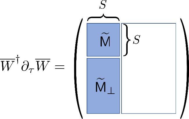
Figure 1. Schematics for the structure of the matrices $\widetilde{{\mathsf{M}}}$ and ${\widetilde{{\mathsf{M}}}}_{\perp }$. |
We now discuss the computational complexity of the effective equations. In the coordinate representation, if L is the number of spatial grids, φ, $\bar{\varphi },$ and η are all vectors with L elements, and ${ \mathcal G }$, ${ \mathcal F }$, ${ \mathcal E },$ and Δ are L × L matrices. As can be seen, the computational complexities of the effective equations and the full Gaussian-state equations (16 ) and (21 ) are O(S × L) and O(L2), respectively. Therefore, the effective-equation approach can be much more efficient when S is small.
4.1. Explicit effective equations for the simplest systems
As the preliminary validity check to EGST, here we derive the explicit equations for the systems with at most one squeezed mode. Specifically, we first consider a pure coherent state, i.e., S = 0. Consequently, equation (46 ) reduces to
$\begin{eqnarray}\begin{array}{rcl}{\partial }_{\tau }\phi ({\boldsymbol{r}}) & = & -\eta ({\boldsymbol{r}})\\ & = & -\left[{h}_{0}+\int {\rm{d}}{\boldsymbol{r}}^{\prime} U({\boldsymbol{r}}-{{\boldsymbol{r}}}{^{\prime} })| \phi ({{\boldsymbol{r}}}{^{\prime} }){| }^{2}+\displaystyle \frac{{g}_{3}}{2}| \phi ({\boldsymbol{r}}){| }^{4}\right]\phi ({\boldsymbol{r}}),\end{array}\end{eqnarray}$
which is exactly the imaginary-time Gross-Pitaevskii equation.We then consider the squeezed coherent state for which only one squeezed mode is macroscopically occupied. Therefore, we take S = 1 and Ns,1 ≫ 1. In addition, the normal and anomalous correlation functions reduce to ${ \mathcal G }({\boldsymbol{r}},{{\boldsymbol{r}}}^{{\prime} })={\varphi }_{1}({\boldsymbol{r}}){\varphi }_{1}^{* }({{\boldsymbol{r}}}^{{\prime} })$ and ${ \mathcal F }({\boldsymbol{r}},{{\boldsymbol{r}}}^{{\prime} })\approx {\varphi }_{1}({\boldsymbol{r}}){\varphi }_{1}({{\boldsymbol{r}}}^{{\prime} })$, respectively, where ${\varphi }_{1}({\boldsymbol{r}})\equiv \sinh {d}_{1}{\bar{\varphi }}_{1}({\boldsymbol{r}})=\sqrt{{N}_{s,1}}{\bar{\varphi }}_{1}({\boldsymbol{r}})$ is the unnormalized squeezed mode function, and we have used the approximation $\coth {d}_{1}\approx 1$ for Ns,1 ≫ 1. Making use of ${\partial }_{\tau }{\varphi }_{1}=\cosh {d}_{1}{\bar{\varphi }}_{1}{\partial }_{\tau }{d}_{1}+\sinh {d}_{1}{\partial }_{\tau }{\bar{\varphi }}_{1}$, the effective equations reduce to48 ), we have ignored terms of the order of or higher than $O({N}_{s,1}^{-1})$. Although equations (48) look different from the squeezed-coherent-state GPEs derived in [32], i.e.,48a ), we may assume that 50 ) back into (51 ), we find 48b ) leads to ηs(r) = 0. The difference of these two sets of equations can be understood by noting that equation (48) is obtained via the imaginary-time evolution of the Gaussian state, while equation (49) is derived through the imaginary-time evolution of the mode functions.
$\begin{eqnarray}\begin{array}{rcl}{\partial }_{\tau }\phi ({\boldsymbol{r}}) & = & -2{\varphi }_{1}({\boldsymbol{r}})\int {\rm{d}}{{\boldsymbol{r}}}^{{\prime} }\\ & & \times \,\left[\right.{\varphi }_{1}^{* }({{\boldsymbol{r}}}^{{\prime} })\eta ({{\boldsymbol{r}}}^{{\prime} })+{\varphi }_{1}({{\boldsymbol{r}}}^{{\prime} }){\eta }^{* }({{\boldsymbol{r}}}^{{\prime} })\left]\right.-\eta ({\boldsymbol{r}}),\end{array}\end{eqnarray}$
$\begin{eqnarray}\begin{array}{rcl}{\partial }_{\tau }{\varphi }_{1}({\boldsymbol{r}}) & = & -{\varphi }_{1}({\boldsymbol{r}})\displaystyle \int {\rm{d}}{{\boldsymbol{r}}}^{{\prime} }\\ & & \times \,\left[\right.{\varphi }_{1}^{* }({{\boldsymbol{r}}}^{{\prime} }){\eta }_{s}({{\boldsymbol{r}}}^{{\prime} })+{\varphi }_{1}({{\boldsymbol{r}}}^{{\prime} }){\eta }_{s}^{* }({{\boldsymbol{r}}}^{{\prime} })\left]\right.-{\eta }_{s}({\boldsymbol{r}}),\end{array}\end{eqnarray}$
where ${\eta }_{s}({\boldsymbol{r}})\equiv \int {\rm{d}}{{\boldsymbol{r}}}^{{\prime} }\left[\right.{ \mathcal E }({\boldsymbol{r}},{{\boldsymbol{r}}}^{{\prime} }){\varphi }_{1}({{\boldsymbol{r}}}^{{\prime} })+{\rm{\Delta }}({\boldsymbol{r}},{{\boldsymbol{r}}}^{{\prime} }){\varphi }_{1}^{* }({{\boldsymbol{r}}}^{{\prime} })\left]\right.$ and to obtain equation ( $\begin{eqnarray}\begin{array}{rc}{\partial }_{\tau }\phi ({\boldsymbol{r}}) & =-\eta ({\boldsymbol{r}}),\end{array}\end{eqnarray}$
$\begin{eqnarray}\begin{array}{rc}{\partial }_{\tau }{\varphi }_{1}({\boldsymbol{r}}) & =-{\eta }_{s}({\boldsymbol{r}}),\end{array}\end{eqnarray}$
we show that equations (48) and (49) give rise to the same (ground) steady state. To this end, we first note that a steady-state solution of equation (49) leads to the relations η(r) = ηs(r) = 0, which obviously satisfy the steady-state condition of equation (48). Conversely, for the steady-state solution of equation ( $\begin{eqnarray}\begin{array}{r}\eta ({\boldsymbol{r}})=\alpha {\bar{\varphi }}_{1}({\boldsymbol{r}}),\end{array}\end{eqnarray}$
where $\begin{eqnarray}\begin{array}{r}\alpha =-2\displaystyle \int {\rm{d}}{{\boldsymbol{r}}}^{{\prime} }\left[\right.{\varphi }_{1}^{* }({{\boldsymbol{r}}}^{{\prime} })\eta ({{\boldsymbol{r}}}^{{\prime} })+{\varphi }_{1}({{\boldsymbol{r}}}^{{\prime} }){\eta }^{* }({{\boldsymbol{r}}}^{{\prime} })\left]\right.\end{array}\end{eqnarray}$
is a real constant. After substituting equation ( $\begin{eqnarray}\begin{array}{r}\alpha =-4{N}_{s,1}\alpha ,\end{array}\end{eqnarray}$
which holds only when α = 0 since Ns,1 > 0. As a result, we obtain η(r) = 0. Similarly, it can also be shown that the steady-state solution of equation (5. Self-bound droplets of dipolar condensates
As a demonstration of EGST, here we revisit the self-bound droplets of dipolar condensates. In the second-quantized form, the Hamiltonian of the system takes the form 40 ), (45 ), and (46 ) to obtain the ground-state wave function. The total energy can then be calculated as E = Ekin + E2B + E3B, where
$\begin{eqnarray}\begin{array}{rcl}\widehat{H} & = & \displaystyle \int {\rm{d}}{\boldsymbol{r}}{\widehat{\psi }}^{\dagger }({\boldsymbol{r}}){h}_{0}\widehat{\psi }({\boldsymbol{r}})\\ & & +\frac{1}{2}\displaystyle \int {\rm{d}}{\boldsymbol{r}}{\rm{d}}{{\boldsymbol{r}}}^{{\prime} }{\widehat{\psi }}^{\dagger }({\boldsymbol{r}}){\widehat{\psi }}^{\dagger }({{\boldsymbol{r}}}^{{\prime} })U({\boldsymbol{r}}-{{\boldsymbol{r}}}^{{\prime} })\widehat{\psi }({{\boldsymbol{r}}}^{{\prime} })\widehat{\psi }({\boldsymbol{r}})\\ & & +\frac{{g}_{3}}{3!}\displaystyle \int {\rm{d}}{\boldsymbol{r}}{\widehat{\psi }}^{\dagger 3}({\boldsymbol{r}}){\widehat{\psi }}^{3}({\boldsymbol{r}}),\end{array}\end{eqnarray}$
where h0 = - ℏ2∇2/(2M) - μ with M being the mass of the atoms and μ the chemical potential. The two-body interaction potential is $\begin{eqnarray}\begin{array}{r}U({\boldsymbol{r}})=\frac{4\pi {\hslash }^{2}{a}_{s}}{M}\delta ({\boldsymbol{r}})+\frac{{\mu }_{0}{\mu }^{2}}{4\pi }\frac{1-3{\cos }^{2}{\theta }_{{\boldsymbol{r}}}}{{r}^{3}},\end{array}\end{eqnarray}$
consisting of the contact and the dipolar interactions, with as being the s-wave scattering length, μ0 the vacuum permeability, μ the magnetic dipole moment of the atom, and θr the polar angle of r. For convenience, we introduce ϵdd = add/as to measure the relative strength of the dipolar interaction with respect to the contact interaction, where add = μ0μ2M/(12πℏ2) is the dipolar length. For the three-body interaction, g3 represents the three-body coupling constant. After applying Wick's theorem, we obtain [32] $\begin{eqnarray}\begin{array}{rcl}\eta & = & {h}_{0}\phi ({\boldsymbol{r}})+\displaystyle \int {\rm{d}}{\boldsymbol{r}}^{\prime} U({\boldsymbol{r}}-{{\boldsymbol{r}}}^{{\prime} })\\ & & \times \left\{\right.\left[\right.| \phi ({{\boldsymbol{r}}}^{{\prime} }){| }^{2}+{ \mathcal G }({{\boldsymbol{r}}}^{{\prime} },{{\boldsymbol{r}}}^{{\prime} })\left]\right.\\ & & \times \phi ({\boldsymbol{r}})+{ \mathcal G }({\boldsymbol{r}},{{\boldsymbol{r}}}^{{\prime} })\phi ({{\boldsymbol{r}}}^{{\prime} })+{ \mathcal F }({\boldsymbol{r}},{{\boldsymbol{r}}}^{{\prime} }){\phi }^{* }({{\boldsymbol{r}}}^{{\prime} })\left\}\right.\\ & & +{g}_{3}\{\left[\right.\frac{1}{2}{\left|\phi ({\boldsymbol{r}})\right|}^{4}+\frac{1}{2}{{ \mathcal F }}^{* }({\boldsymbol{r}},{\boldsymbol{r}}){\phi }^{2}({\boldsymbol{r}})\\ & & +\frac{3}{2}| { \mathcal F }({\boldsymbol{r}},{\boldsymbol{r}}){| }^{2}+3{ \mathcal G }({\boldsymbol{r}},{\boldsymbol{r}})\\ & & \times \left({\left|\phi ({\boldsymbol{r}})\right|}^{2}+{ \mathcal G }({\boldsymbol{r}},{\boldsymbol{r}})\right)\left]\right.\phi ({\boldsymbol{r}})\\ & & +3\left[\frac{1}{2}| \phi ({\boldsymbol{r}}){| }^{2}+{ \mathcal G }({\boldsymbol{r}},{\boldsymbol{r}})\right]{ \mathcal F }({\boldsymbol{r}},{\boldsymbol{r}}){\phi }^{* }({\boldsymbol{r}})\},\,\end{array}\end{eqnarray}$
$\begin{eqnarray}\begin{array}{rcl}{ \mathcal E } & = & {h}_{0}+\delta ({\boldsymbol{r}}-{{\boldsymbol{r}}}^{{\rm{{\prime} }}})\displaystyle \int {\rm{d}}{{\boldsymbol{r}}}_{1}U({\boldsymbol{r}}-{{\boldsymbol{r}}}_{1})\\ & & \times \left[|\phi ({{\boldsymbol{r}}}_{1}){|}^{2}+{ \mathcal G }({{\boldsymbol{r}}}_{1},{{\boldsymbol{r}}}_{1})\right]+U({\boldsymbol{r}}-{{\boldsymbol{r}}}^{{\rm{{\prime} }}})[{\phi }^{\ast }({{\boldsymbol{r}}}^{{\rm{{\prime} }}})\phi ({\boldsymbol{r}})+{ \mathcal G }({\boldsymbol{r}},{{\boldsymbol{r}}}^{{\rm{{\prime} }}})]\\ & & +\frac{3}{2}{g}_{3}\delta ({\boldsymbol{r}}-{{\boldsymbol{r}}}^{{\rm{{\prime} }}})\left[|\phi ({\boldsymbol{r}}){|}^{4}+4|\phi ({\boldsymbol{r}}){|}^{2}{ \mathcal G }({\boldsymbol{r}},{\boldsymbol{r}})\right.\\ & & \left.+2{\rm{Re}}{{ \mathcal F }}^{\ast }({\boldsymbol{r}},{\boldsymbol{r}}){\phi }^{2}({\boldsymbol{r}})+2{ \mathcal G }{({\boldsymbol{r}},{\boldsymbol{r}})}^{2}+|{ \mathcal F }({\boldsymbol{r}},{\boldsymbol{r}}){|}^{2}\right],\end{array}\end{eqnarray}$
$\begin{eqnarray}\begin{array}{rcl}{\rm{\Delta }} & = & U({\boldsymbol{r}}-{{\boldsymbol{r}}}^{{\prime} })[\phi ({{\boldsymbol{r}}}^{{\prime} })\phi ({\boldsymbol{r}})+{ \mathcal F }({\boldsymbol{r}},{{\boldsymbol{r}}}^{{\prime} })]\\ & & +{g}_{3}\delta ({\boldsymbol{r}}-{{\boldsymbol{r}}}^{{\prime} })\left[| \phi ({\boldsymbol{r}}){| }^{2}\phi {({\boldsymbol{r}})}^{2}\right.\\ & & +3\phi {({\boldsymbol{r}})}^{2}{ \mathcal G }({\boldsymbol{r}},{\boldsymbol{r}})+3| \phi ({\boldsymbol{r}}){| }^{2}{ \mathcal F }({\boldsymbol{r}},{\boldsymbol{r}})\\ & & \left.+3{ \mathcal G }({\boldsymbol{r}},{\boldsymbol{r}}){ \mathcal F }({\boldsymbol{r}},{\boldsymbol{r}})\right],\,\end{array}\end{eqnarray}$
where ${ \mathcal G }({\boldsymbol{r}},{{\boldsymbol{r}}}^{{\prime} })={\sum }_{j=1}^{S}{\sinh }^{2}{d}_{j}{\bar{\varphi }}_{j}^{* }({{\boldsymbol{r}}}^{{\prime} }){\bar{\varphi }}_{j}({\boldsymbol{r}})$ and ${ \mathcal F }({\boldsymbol{r}},{{\boldsymbol{r}}}^{{\prime} })\,={\sum }_{j=1}^{S}\sinh {d}_{j}\cosh {d}_{j}{\bar{\varphi }}_{j}({{\boldsymbol{r}}}^{{\prime} }){\bar{\varphi }}_{j}({\boldsymbol{r}})$. With these quantities specified, one can then numerically evolve the effective equations ( $\begin{eqnarray}\begin{array}{rcl}{E}_{{\rm{kin}}} & = & \displaystyle \int {\rm{d}}{\boldsymbol{r}}\left[{\phi }^{* }({\boldsymbol{r}}){h}_{0}({\boldsymbol{r}})\phi ({\boldsymbol{r}})\right.\\ & & \left.+\displaystyle \sum _{j=1}^{S}{\sinh }^{2}{d}_{j}{\bar{\varphi }}_{j}^{* }({\boldsymbol{r}}){h}_{0}({\boldsymbol{r}}){\bar{\varphi }}_{j}({\boldsymbol{r}})\right],\end{array}\end{eqnarray}$
$\begin{eqnarray}\begin{array}{rcl}{E}_{2B} & = & \displaystyle \int {\rm{d}}{\boldsymbol{r}}{\rm{d}}{\boldsymbol{r}}^{\prime} U({\boldsymbol{r}}-{{\boldsymbol{r}}}^{{\prime} })\left\{\right.\frac{1}{2}| \phi ({\boldsymbol{r}}){| }^{2}| \phi ({{\boldsymbol{r}}}^{{\prime} }){| }^{2}\\ & & +{ \mathcal G }({\boldsymbol{r}},{\boldsymbol{r}})\left[\right.| \phi ({{\boldsymbol{r}}}^{{\prime} }){| }^{2}+\frac{1}{2}{ \mathcal G }({{\boldsymbol{r}}}^{{\prime} },{{\boldsymbol{r}}}^{{\prime} })\left]\right.\\ & & +{ \mathcal G }({{\boldsymbol{r}}}^{{\prime} },{\boldsymbol{r}})\left[\right.\phi ({\boldsymbol{r}}){\phi }^{* }({{\boldsymbol{r}}}^{{\prime} })+\frac{1}{2}{ \mathcal G }({\boldsymbol{r}},{{\boldsymbol{r}}}^{{\prime} })\left]\right.\\ & & +{\rm{Re}}{{ \mathcal F }}^{* }({\boldsymbol{r}},{{\boldsymbol{r}}}^{{\prime} })\left[\right.\phi ({\boldsymbol{r}})\phi ({{\boldsymbol{r}}}^{{\prime} })+\frac{1}{2}{ \mathcal F }({\boldsymbol{r}},{{\boldsymbol{r}}}^{{\prime} })\left]\right.\left\}\right.,\end{array}\end{eqnarray}$
and $\begin{eqnarray}\begin{array}{rcl}{E}_{3B} & = & {g}_{3}\displaystyle \int {\rm{d}}{\boldsymbol{r}}\left[\frac{1}{3!}| \phi ({\boldsymbol{r}}){| }^{6}+\frac{3}{2}| \phi ({\boldsymbol{r}}){| }^{4}{ \mathcal G }({\boldsymbol{r}},{\boldsymbol{r}})\right.\\ & & +{\rm{Re}}| \phi ({\boldsymbol{r}}){| }^{2}{\phi }^{2}({\boldsymbol{r}}){{ \mathcal F }}^{* }({\boldsymbol{r}},{\boldsymbol{r}})+3| \phi ({\boldsymbol{r}}){| }^{2}{{ \mathcal G }}^{2}({\boldsymbol{r}},{\boldsymbol{r}})\\ & & +3{\rm{Re}}{\phi }^{2}({\boldsymbol{r}}){{ \mathcal F }}^{* }({\boldsymbol{r}},{\boldsymbol{r}}){ \mathcal G }({\boldsymbol{r}},{\boldsymbol{r}})+\frac{3}{2}| \phi ({\boldsymbol{r}}){| }^{2}| { \mathcal F }({\boldsymbol{r}},{\boldsymbol{r}}){| }^{2}\\ & & \left.+\frac{3}{2}{ \mathcal G }({\boldsymbol{r}},{\boldsymbol{r}})| { \mathcal F }({\boldsymbol{r}},{\boldsymbol{r}}){| }^{2}+{{ \mathcal G }}^{3}({\boldsymbol{r}},{\boldsymbol{r}})\right]\end{array}\end{eqnarray}$
are, respectively, the kinetic, two-body interaction, and three-body interaction energies. In addition, we can further compute the total density n(r) = nc(r) + ns(r), where nc(r) = ∣φ(r)∣2 and ${n}_{s}({\boldsymbol{r}})={\sum }_{j=1}^{S}{\sinh }^{2}{d}_{j}| {\bar{\varphi }}_{j}({\boldsymbol{r}}){| }^{2}$ are, respectively, the densities of the coherent and squeezed atoms. We note that all densities are axially symmetric due to the cylindrical symmetry of the dipolar interaction.As a concrete example, we consider a condensate of N = 103 dysprosium atoms, each possessing a magnetic dipole moment of μ = 10μB, with μB being the Bohr magneton. Since the scattering length as is tunable via Feshbach resonance, we treat as, or equivalently ϵdd, as a free parameter. More specifically, we shall focus on the regime with ϵdd > 1.23, because the condensate becomes self-bound only in this regime [32]. For the three-body coupling strength, we adopt the value used in Reference [32], i.e., g3 = 6.73 × 10-40ℏm6/s. Previously, the full GST showed that, by increasing ϵdd, the condensate falls into the SVS, SCS, and CS phases sequentially [32]. The phase boundaries are located at ϵdd = 1.33 and 1.79. Finally, for convenience, we shall refer to the results obtained from the effective theory as approximate results and those from the full GST as exact results.
To validate EGST, we consider the case with ϵdd = 2. In figure 2(a), we plot the S dependence of the total energy E and the coherent atom fraction fc. Next, in figure 2(b), we plot the S dependence of the condensate radial size ${\sigma }_{\rho }={\left[\int {\rm{d}}{\boldsymbol{r}}{\rho }^{2}n({\boldsymbol{r}})\right]}^{1/2}$ and the peak density npeak. Here the peak density npeak is the maximal value of n(r), and we find under all circumstances that npeak = n(0). Finally, figure 2(c) shows the S dependence of the occupation numbers in the first four squeezed modes. As can be seen, all physical quantities converge to the corresponding exact values when S is roughly over Sconv = 50, which seems quite large. This, however, is not completely unexpected, since, for the given parameter, the system lies deep inside the CS phase which involves many squeezed modes. As shall be shown, the situation can be greatly improved in the SVS and SCS phases.
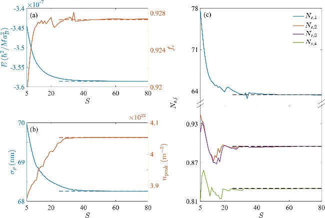
Figure 2. (a) Total energy and coherent fraction, (b) radial width and peak density, and (c) occupation numbers in the four most hightly populated squeezed modes, as functions of the number of the effective squeezed modes for N = 1000 and ϵdd = 2. The dashed lines denote the corresponding result computed via the full GST. |
For a more detailed comparison, in figure 3, we plot the approximate densities of the coherent and squeezed atoms along both radial and axial directions for ϵdd = 2 and different values of S. As a comparison, we also plot the exact densities in the corresponding figures. As can be seen, all approximate densities roughly converge to the exact ones for S = 40, which confirms the observation in figure 2.
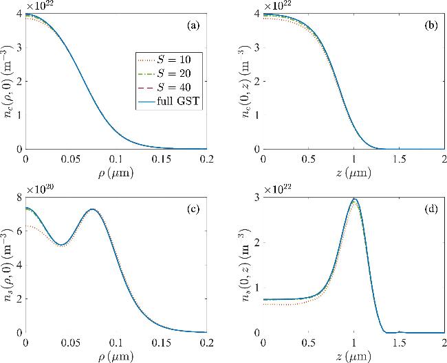
Figure 3. Approximate density profiles (a) nc(ρ, 0), (b) nc(0, z), (c) ns(ρ, 0), and (d) ns(0, z) for ϵdd = 2 where N = 1000 under various cutoff numbers S = 10 (dotted lines), 20 (dash-dotted lines), and 40 (dashed lines). Solid lines show the results from the full GST calculations. |
Finally, to see the convergence in other quantum phases, we plot in figure 4 the error of the total energy, i.e., ΔE = Eapproximate - Eexact as a function of ϵdd for various S's. As expected, ΔE monotonically decreases with the increase of S throughout the interaction regime. In addition, for a given S, ΔE monotonically increases with ϵdd. More specifically, in the SVS phase, it is found that the solutions roughly converge for S = 10. However, across the whole SCS phase, S has to be as large as 40 to ensure the convergence of the solution. The required cutoff becomes even larger in the CS phase, where, as shown in figure 2, Sconv increases to 50. Therefore, substantial efficiency can be gained from the effective equations mainly in the SVS and SCS phases.
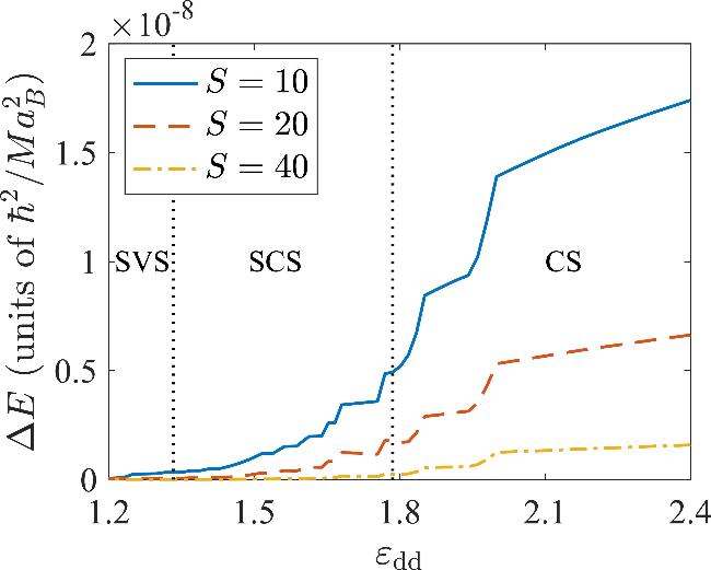


Figure 4. Error of the total energy as a function of ϵdd for S = 10 (solid line), 20 (dashed line), and 40 (dash-dotted line). |
6. Conclusions
In conclusion, we have developed an effective-equation approach for GST by deriving the imaginary-time evolution equations for the squeezed modes and the occupation numbers. We have validated these effective equations using a dipolar droplet system. The results obtained from the effective equations converge to those of the full GST when the number of squeezed modes included in the calculation is sufficiently large, confirming the accuracy of the approach. Since the effective equations involve only the retained squeezed modes, the approach can be numerically more efficient than the full GST. In particular, for the SVS and SCS phases of dipolar droplets, in which the number of notably occupied squeezed modes is small, the effective equation approach has a substantial advantage.