

1. Introduction
The mid-infrared (MIR) or far-infrared (FIR) frequency ranges, spanning several to hundreds of terahertz (wavelengths from 2.5 to 500 $\mu$m), constitute a crucial part of the electromagnetic spectrum and underpin a broad range of applications. These include molecular analysis of biological tissues [1], clinical medicine [1], thermal imaging [2], quantum sensing [3], microscopy [4, 5], astronomy [6, 7], and homeland security. Infrared (IR) detectors are crucial to these applications. Conventional IR detectors are highly sensitive to thermal noise and typically require cryogenic cooling to mitigate thermal interference. This need for cryogenic cooling makes these detectors both costly and less sensitive compared with visible (VIS) [or near-infrared (NIR)] detectors. These limitations highlight the urgent need for IR detection technologies that are compact, highly sensitive, and low-noise, while operating without complex cryogenic systems.
A promising approach for detecting MIR and FIR signals is to upconvert them into the VIS (or NIR) range, where compact, cost-effective, and highly sensitive cameras are readily available. Existing coherent conversion methods include nonlinear interferometry [8, 9] and frequency upconversion [10-14]. In nonlinear interferometry, IR signals are upconverted into VIS (or NIR) light through three-wave mixing in bulk nonlinear crystals. And its efficient upconversion requires stringent phase matching among the IR, pump, and upconverted fields during propagation [15, 16]. Inspired by advances in cavity optomechanics that enable coherent frequency conversion [17-30], another approach for IR signal detection employs plasmonic nanocavities containing molecules with both IR-absorption and Raman-active vibrational modes to upconvert MIR (or FIR) signals into the VIS (or NIR) range [11]. Subsequently, experiments demonstrated that plasmonic nanocavities containing hundreds of biphenyl-4-thiol molecules can achieve IR-to-VIS conversion at room temperature [12, 13]. Yet the low conversion efficiency poses a significant challenge for the applications of such a mechanism of upconversion.
To enhance conversion efficiency, we recently proposed an amplification mechanism based on molecular collective mode and Stokes sideband pumping in the molecular optomechanical system [14]. This scheme has the potential to increase the intensity by a factor of 1000 or more for the IR signal without considering the impact of noise. A more comprehensive investigation is needed to evaluate the impact of system noise on IR signal detection and to quantify the resulting output noise levels.
In this work, we employ the power spectrum method [31, 32] to investigate the properties of the upconverted IR signals in a molecular optomechanical cavity under both red- and blue-detuned conditions, where the driving frequency equals the sum or difference of the VIS and vibrational frequencies. This method allows us to analyze the conversion efficiency from IR signal to VIS range, as well as the noise added to the upconverted signal. We analyze the conversion efficiencies at both the first Stokes and anti-Stokes sidebands of the pump field. These results indicate that under the red-detuned condition, the anti-Stokes sideband exhibits higher conversion efficiency than the Stokes sideband; the opposite occurs under the blue-detuned condition, where amplification of the IR signal is achieved. Additionally, we analyze how the system parameters affect both the conversion efficiency and the noise added to the upconverted signal. It is shown that the added noise is suppressed by appropriately tuning the coupling strength and decay rates of the system. These findings provide a theoretical foundation for future experimental advances in IR signal upconversion.
2. Molecular optomechanical system
We consider a molecular optomechanical system [33-51] consisting of $N$ identical molecules and a plasmonic nanocavity that supports both the VIS and IR modes (figure 1(a)). As depicted in figure 1(b), the plasmonic nanocavity is realized through a nanoparticle-on-resonator configuration, where an Au nanoparticle is positioned on top of an Au disk, with the $N$ identical molecules placed in the gap between the nanoparticle and the disk [13, 51]. In the low-excitation limit of the molecular vibrations, the vibrational mode of each molecule is approximately modeled as a harmonic oscillator [33]. To achieve frequency upconversion of the IR signal of interest, particular types of molecules, e.g. Biphenyl-4-thiol [12, 13], are selected to couple simultaneously to both the VIS and IR modes within the plasmonic nanocavity. Due to the negligibly small dipole moment of Biphenyl-4-thiol molecules, intermolecular interactions can be safely neglected compared with the interactions between the VIS (IR) mode and the molecular vibrations. A strong pump field in the VIS range, with frequency $\omega_{p}$ and amplitude $\varepsilon_{p}$, is applied to drive the VIS mode within the nanocavity. The Hamiltonian of the system is given as ($\hbar = 1$) [14]
$\begin{align} H_{s} & = \omega_{a}a^{\dagger}a+\omega_{c}c^{\dagger}c+\sum_{j = 1}^{N}\omega_{b}b_{j}^{\dagger}b_{j}+\sum_{j = 1}^{N}g_{a}a^{\dagger}a\left(b_{j}^{\dagger}+b_{j}\right)\nonumber \\ & \quad+\sum_{j = 1}^{N}g_{c}\left(c^{\dagger}+c\right)\left(b_{j}^{\dagger}+b_{j}\right)+{\mathrm{i}}\left(\varepsilon_{p}\text{e}^{-{\mathrm{i}}\omega_{p}t}a^{\dagger}-\mathrm{H.c.}\right),\end{align}$
where $a$ ($a^{\dagger}$) and $c$ ($c^{\dagger}$) represent the annihilation (creation) operators for the VIS and IR modes with resonance frequencies $\omega_{a}$ and $\omega_{c}$, respectively. The operator $b_{j}$ ($b_{j}^{\dagger}$) is the annihilation (creation) operator for the vibrational mode of the $j$th molecule with resonance frequency $\omega_{b}$. The parameter $g_{a}$ denotes the optomechanical coupling strength between the VIS mode of the cavity and the molecular vibrations, arising from the dispersive interaction mediated by the Raman polarizability [33, 52-57]. In contrast, $g_{c}$ represents the bilinear coupling strength between the IR mode and the molecular vibrations, which originates from the electric-dipole interaction [11, 58, 59]. Here, we assume that the coupling strengths between the VIS (IR) mode and the molecular vibrations are identical for all molecules, which is valid when the size of the molecular ensemble is sufficiently small compared with the spatial variation scale of the cavity modes. For simplicity but without loss of generality, we assume that the parameters $g_{a}$, $g_{c}$, and $\varepsilon_{p}$ are real. Instead of adding explicit form of IR signal of interest [14], we will treat the IR signal as part of the input of the cavity IR mode following the standard power spectrum methods [31, 32] in the following discussions.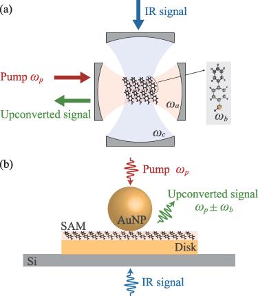
Figure 1. (a) Schematic diagram of a molecular optomechanical system, where the molecular vibrations are coupled to the VIS (IR) mode of the cavity via dispersive (electric-dipole) interaction. A strong pump field with frequency $\omega_{p}$ is applied to drive the VIS mode within the cavity. (b) Schematic diagram of a nanoparticle-on-resonator configuration. From top to bottom, it consists of an Au nanoparticle (AuNP), a self-assembled monolayer (SAM) of Biphenyl-4-thiol, an Au disk, and a Si layer. |
We introduce the molecular collective operator $B = \sum_{j = 1}^{N}b_{j}/\sqrt{N}$, which satisfies the bosonic commutation relation $[B,B^{\dagger}] = 1$. In the interaction picture with respect to $\omega_{p}a^{\dagger}a$, Hamiltonian (1) is simplified as
$\begin{align} H & = \Delta_{0}a^{\dagger}a+\omega_{c}c^{\dagger}c+\omega_{b}B^{\dagger}B+G_{a}a^{\dagger}a(B^{\dagger}+B)\nonumber \\ & \quad+G_{c}(c^{\dagger}+c)(B^{\dagger}+B)+{\mathrm{i}}(\varepsilon_{p}a^{\dagger}-\mathrm{H.c.)},\end{align}$
where $\Delta_{0} = \omega_{a}-\omega_{p}$ is the detuning between the VIS mode and the pump field. The parameters $G_{a} = g_{a}\sqrt{N}$ and $G_{c} = g_{c}\sqrt{N}$ represent the collective optomechanical coupling strength and the collective bilinear coupling strength, respectively.By substituting Hamiltonian (2 ) into the Heisenberg equation and accounting for the damping and the corresponding noise terms, the quantum Langevin equations (QLEs) are obtained as follows:
$\begin{align} \dot{a} & = -\left({\mathrm{i}}\Delta_{0}+\kappa_{a}\right)a-{\mathrm{i}}G_{a}a\left(B^{\dagger}+B\right)+\varepsilon_{p}+\sqrt{2\kappa_{a}}a_{\mathrm{in}},\nonumber \\ \dot{c} & = -\left({\mathrm{i}}\omega_{c}+\kappa_{c}\right)c-{\mathrm{i}}G_{c}\left(B^{\dagger}+B\right)+\sqrt{2\kappa_{c}}c_{\mathrm{in}},\nonumber \\ \dot{B} & = -\left({\mathrm{i}}\omega_{b}+\gamma_{B}\right)B-{\mathrm{i}}G_{a}a^{\dagger}a-{\mathrm{i}}G_{c}\left(c^{\dagger}+c\right)+\sqrt{2\gamma_{B}}B_{\mathrm{in}}\nonumber,\end{align}$
where $\kappa_{a}$ and $\kappa_{c}$ are the decay rates of the VIS and IR modes, respectively, and $\gamma_{B}$ is the decay rate of the molecular collective mode. Note that we consider a single-sided cavity damping scenario, and neglect the intrinsic decay of both the VIS and IR modes. The operators $a_{\mathrm{in}}$, $c_{\mathrm{in}}$, and $B_{\mathrm{in}} = \sum_{j = 1}^{N}b_{j,\mathrm{in}}/\sqrt{N}$ represent the inputs, including both vacuum thermal noise and possible external coherent input. In the absence of coherent input, these operators have zero mean values $\langle o_{\mathrm{in}}\rangle = 0$ and nonzero correlation functions given by $\langle o_{\mathrm{in}}^{\dagger}(t)o_{\mathrm{in}}(t^{^{\prime}})\rangle = n_{o}^{\mathrm{th}}\delta(t-t^{^{\prime}})\approx0$ and $\langle o_{\mathrm{in}}(t)o_{\mathrm{in}}^{\dagger}(t^{^{\prime}})\rangle = (n_{o}^{\mathrm{th}}+1)\delta(t-t^{^{\prime}})\approx\delta(t-t^{^{\prime}})$ for $o = a,c,B$. Here we assume the thermal occupations $n_{a,c,B}^{\mathrm{th}} = 1/[\exp(\hbar\omega_{a,c,b}/k_{\mathrm{B}}T)-1]$ of the VIS and IR modes as well as the molecular vibrational mode are negligible due to $\hbar\omega_{a,c,b}/k_{\mathrm{B}}T\gg1$, where $k_{\mathrm{B}}$ is the Boltzmann constant and $T$ is the ambient temperature (e.g. $300$ K), i.e. $n_{a,c,B}^{\mathrm{th}}\approx0$.Here, we would like to remark on the treatment of the input $c_{\mathrm{in}}$. Without any coherent input, we treat $c_{\mathrm{in}}$ as the vacuum thermal noise with zero mean values $\langle c_{\mathrm{in}}\rangle = 0$ to obtain the steady state. And the later response in the VIS signal is then evaluated by treating the input $c_{\mathrm{in}}$ as the sum of the coherent input and vacuum thermal noise.
Under the condition of a strong pump field, the steady-state mean values of the operators are obtained using the mean-field approximation, where $\left\langle a^{\dagger}a\right\rangle _{\mathrm{ss}}\approx\left\langle a^{\dagger}\right\rangle _{\mathrm{ss}}\left\langle a\right\rangle _{\mathrm{ss}}$, yielding
$\begin{align} \langle a\rangle_{\mathrm{ss}} & = \frac{\varepsilon_{p}}{{\mathrm{i}}\Delta+\kappa_{a}},\nonumber \\ \langle c\rangle_{\mathrm{ss}} & = -\frac{{\mathrm{i}}G_{c}\left(\langle B\rangle_{\mathrm{ss}}^{*}+\langle B\rangle_{\mathrm{ss}}\right)}{{\mathrm{i}}\omega_{c}+\kappa_{c}},\nonumber \\ \langle B\rangle_{\mathrm{ss}} & = -\frac{{\mathrm{i}}\left[G_{a}|\langle a\rangle_{\mathrm{ss}}|^{2}+G_{c}\left(\langle c\rangle_{\mathrm{ss}}^{*}+\langle c\rangle_{\mathrm{ss}}\right)\right]}{{\mathrm{i}}\omega_{b}+\gamma_{B}},\end{align}$
where $\Delta = \Delta_{0}+G_{a}(\langle B\rangle_{\mathrm{ss}}^{*}+\langle B\rangle_{\mathrm{ss}})$ is the effective detuning. Note that the strong driving regime refers to the condition where the steady-state field amplitude satisfies $\left|\left\langle a\right\rangle_{\mathrm{ss}}\right|\gg1$, such that the effect of the quantum fluctuation around the mean field is negligible.With the strong pump field, each operator is rewritten as the sum of the steady-state mean value and the quantum fluctuation, i.e. $o = \langle o\rangle_{\mathrm{ss}}+\delta o$ for $o = a,c,B$ [60]. By keeping only the first-order term of the quantum fluctuation, the linearized QLEs are obtained as 5 ), the linearized effective Hamiltonian is written as 5 ).
$\begin{align} \delta\dot{a} & = -\left({\mathrm{i}}\Delta+\kappa_{a}\right)\delta a-{\mathrm{i}}\mathcal{G}_{a}\left(\delta B^{\dagger}+\delta B\right)+\sqrt{2\kappa_{a}}a_{\mathrm{in}},\nonumber \\ \delta\dot{c} & = -\left({\mathrm{i}}\omega_{c}+\kappa_{c}\right)\delta c-{\mathrm{i}}G_{c}\left(\delta B^{\dagger}+\delta B\right)+\sqrt{2\kappa_{c}}c_{\mathrm{in}},\nonumber \\ \delta\dot{B} & = -\left({\mathrm{i}}\omega_{b}+\gamma_{B}\right)\delta B-{\mathrm{i}}\left(\mathcal{G}_{a}^{*}\delta a+\mathcal{G}_{a}\delta a^{\dagger}\right)\nonumber \\ & \quad-{\mathrm{i}}G_{c}\left(\delta c+\delta c^{\dagger}\right)+\sqrt{2\gamma_{B}}B_{\mathrm{in}},\end{align}$
where $\mathcal{G}_{a} = G_{a}\langle a\rangle_{\mathrm{ss}}$ represents the enhanced collective optomechanical coupling strength. According to equation ($\begin{align} H_{\mathrm{eff}} & = \Delta\delta a^{\dagger}\delta a+\omega_{c}\delta c^{\dagger}\delta c+\omega_{b}\delta B^{\dagger}\delta B+\mathcal{G}_{a}\delta a^{\dagger}\left(\delta B^{\dagger}+\delta B\right)\nonumber \\ & \quad+\mathcal{G}_{a}^{*}\delta a\left(\delta B^{\dagger}+\delta B\right)+G_{c}\left(\delta c+\delta c^{\dagger}\right)\left(\delta B^{\dagger}+\delta B\right).\end{align}$
In the following, we use the power spectrum method [31, 32] to solve the linearized QLEs (By defining the fluctuation vector $\mu = (\delta a,\delta c,\delta B,\delta a^{\dagger},\delta c^{\dagger},$ $\delta B^{\dagger})^{\mathrm{T}}$ and the input field vector $\mu_{\mathrm{in}} = (a_{\mathrm{in}},c_{\mathrm{in}},B_{\mathrm{in}},a_{\mathrm{in}}^{\dagger},c_{\mathrm{in}}^{\dagger},B_{\mathrm{in}}^{\dagger})^{\mathrm{T}}$, the linearized QLEs (5 ) is written as
$\begin{align} \frac{{\mathrm{d}}\mu}{{\mathrm{d}}t} = -M\mu+L\mu_{\mathrm{in}},\end{align}$
where $L = \mathrm{diag}(\sqrt{2\kappa_{a}},\sqrt{2\kappa_{c}},\sqrt{2\gamma_{B}},\sqrt{2\kappa_{a}},\sqrt{2\kappa_{c}},\sqrt{2\gamma_{B}})$ is the damping matrix and $M = \left(\begin{array}{cc} P & Q\\ Q^{*} & P^{*} \end{array}\right)$ is the coefficient matrix with $\begin{align} P = \left(\begin{array}{ccc} {\mathrm{i}}\Delta+\kappa_{a} & 0 & {\mathrm{i}}\mathcal{G}_{a}\\ 0 & {\mathrm{i}}\omega_{c}+\kappa_{c} & {\mathrm{i}}G_{c}\\ {\mathrm{i}}\mathcal{G}_{a}^{*} & {\mathrm{i}}G_{c} & {\mathrm{i}}\omega_{b}+\gamma_{B} \end{array}\right),\end{align}$
and $\begin{align} Q = \left(\begin{array}{ccc} 0 & 0 & {\mathrm{i}}\mathcal{G}_{a}\\ 0 & 0 & {\mathrm{i}}G_{c}\\ {\mathrm{i}}\mathcal{G}_{a} & {\mathrm{i}}G_{c} & 0 \end{array}\right).\end{align}$
The system is stable only when the real parts of all the eigenvalues of the coefficient matrix $M$ are positive, as determined by the Routh-Hurwitz criterion [61, 62].Figure 2 illustrates the stability diagram of the system for the blue-detuned pump field with $\Delta = -\omega_{b}$ and the resonance condition with $\omega_{c} = \omega_{b}$. Other parameters are as shown in the caption of figure 2. The results show that the system is stable in the white area. For the red-detuned pump field with $\Delta = \omega_{b}$, the system is entirely stable across the same parameter range (not shown here).
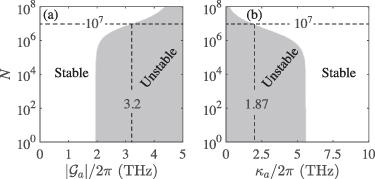
Figure 2. The stability diagram with respect to (a) the enhanced collective optomechanical coupling strength $\left|\mathcal{G}_{a}\right|$ and the number of the molecules $N$ at $\kappa_{a}/2\pi = 30\,\mathrm{THz}$; (b) the decay rate of the VIS mode $\kappa_{a}$ and the number of the molecules $N$ at $|\mathcal{G}_{a}|/2\pi = 0.75\,\mathrm{THz}$. Here we take the blue-detuned case of $\Delta = -\omega_{b}$. Other parameters are $\omega_{b} = \omega_{c} = 2\pi\times30\,\mathrm{THz}$, $g_{c}/2\pi = 0.1\,\mathrm{GHz}$, $\varepsilon_{p}/2\pi = 500\,\mathrm{THz}$, $\gamma_{B}/2\pi = 0.1\,\mathrm{THz}$, and $\kappa_{c}/2\pi = 0.5\,\mathrm{THz}$. |
With the Fourier transform of the operators 7 ) in the frequency domain is 11 ), the output field vector is obtained as
$\begin{align} \tilde{o}\left(\omega\right) & = \frac{1}{\sqrt{2\pi}}\int_{-\infty}^{+\infty}o\left(t\right)\text{e}^{-{\mathrm{i}}\omega t}{\mathrm{d}}t,\nonumber \\ \widetilde{o^{\dagger}}\left(\omega\right) & = \frac{1}{\sqrt{2\pi}}\int_{-\infty}^{+\infty}o^{\dagger}\left(t\right)\text{e}^{-{\mathrm{i}}\omega t}{\mathrm{d}}t,\end{align}$
satisfying $[\tilde{o}(\omega)]^{\dagger} = \widetilde{o^{\dagger}}(-\omega)$, the solution of equation ($\begin{align} \tilde{\mu}\left(\omega\right) = \left(M+{\mathrm{i}}\omega I_{6}\right)^{-1}L\tilde{\mu}_{\mathrm{in}}\left(\omega\right),\end{align}$
where $I_{6}$ represents the $6\times6$ identity matrix, and $\tilde{\mu}(\omega)$ [$\tilde{\mu}_{\mathrm{in}}(\omega)$] denotes the Fourier transform of the vector $\tilde{\mu}$ ($\tilde{\mu}_{\mathrm{in}}$). By substituting the input-output relation $\tilde{\mu}_{\mathrm{out}}(\omega)+\tilde{\mu}_{\mathrm{in}}(\omega) = L\tilde{\mu}(\omega)$ [63] into equation ($\begin{align} \tilde{\mu}_{\mathrm{out}}\left(\omega\right) = U\left(\omega\right)\tilde{\mu}_{\mathrm{in}}\left(\omega\right),\end{align}$
where the scattering matrix $U(\omega)$ is given by $\begin{align} U\left(\omega\right) = L\left(M+{\mathrm{i}}\omega I_{6}\right)^{-1}L-I_{6}.\end{align}$
The matrix element $U_{jj^{^{\prime}}}(\omega)$ is the element in the $j$th row and $j^{^{\prime}}$th column of the scattering matrix $U(\omega)$, and denotes the scattering amplitude from the $j^{^{\prime}}$th component to the $j$th one.$\begin{align} \langle\widetilde{o^{\dagger}}_{\mathrm{in}}\left(\omega\right)\tilde{o}_{\mathrm{in}}\left(\omega^{^{\prime}}\right)\rangle & = S_{o,\mathrm{in}}\left(\omega\right)\delta\left(\omega+\omega^{^{\prime}}\right),\end{align}$
$align$
where $S_{o,\mathrm{in}}(\omega)$ ($o = a,c,B$) denotes the spectrum of coherent input, and the term '1' accounts for the contribution from the vacuum noise. The output spectrum $S_{o,\mathrm{out}}(\omega)$ is defined by [31]$\begin{align} S_{o,\mathrm{out}}\left(\omega\right) = \frac{1}{2}\int_{-\infty}^{\infty}\langle\widetilde{o^{\dagger}}_{\mathrm{out}}\left(\omega\right)\tilde{o}_{\mathrm{out}}\left(\omega^{^{\prime}}\right)+\tilde{o}_{\mathrm{out}}\left(\omega^{^{\prime}}\right)\widetilde{o^{\dagger}}_{\mathrm{out}}\left(\omega\right)\rangle {\mathrm{d}}\omega^{^{\prime}}.\end{align}$
By substituting equations ($\begin{align} S_{\mathrm{out}}\left(\omega\right) = T\left(\omega\right)\left[S_{\mathrm{in}}\left(\omega\right)+\frac{1}{2}\left(\begin{array}{c} 1\\ 1\\ 1 \end{array}\right)\right],\end{align}$
where $S_{\mathrm{out}}(\omega) = (S_{a,\mathrm{out}}(\omega),S_{c,\mathrm{out}}(\omega),S_{B,\mathrm{out}}(\omega))^{\mathrm{T}}$ and $S_{\mathrm{in}}(\omega) = (S_{a,\mathrm{in}}(\omega),S_{c,\mathrm{in}}(\omega),S_{B,\mathrm{in}}(\omega))^{\mathrm{T}}$. The matrix $T(\omega)$ is defined as $\begin{align} T\left(\omega\right) = \left(\begin{array}{ccc} T_{aa}\left(\omega\right) & T_{ac}\left(\omega\right) & T_{aB}\left(\omega\right)\\ T_{ca}\left(\omega\right) & T_{cc}\left(\omega\right) & T_{cB}\left(\omega\right)\\ T_{Ba}\left(\omega\right) & T_{Bc}\left(\omega\right) & T_{BB}\left(\omega\right) \end{array}\right),\end{align}$
where the matrix element $T_{oo^{^{\prime}}}(\omega)$ $\left(o,o^{^{\prime}} = a,c,B\right)$ represents the scattering probability from mode $o^{^{\prime}}$ to mode $o$ with$\begin{align} T_{aa}\left(\omega\right) & = \left|U_{11}\left(\omega\right)\right|^{2}+\left|U_{14}\left(\omega\right)\right|^{2},\end{align}$
$\begin{align} T_{ac}\left(\omega\right) & = \left|U_{12}\left(\omega\right)\right|^{2}+\left|U_{15}\left(\omega\right)\right|^{2},\end{align}$
$\begin{align} T_{aB}\left(\omega\right) & = \left|U_{13}\left(\omega\right)\right|^{2}+\left|U_{16}\left(\omega\right)\right|^{2},\end{align}$
$\begin{align} T_{ca}\left(\omega\right) & = \left|U_{21}\left(\omega\right)\right|^{2}+\left|U_{24}\left(\omega\right)\right|^{2},\end{align}$
$\begin{align} T_{cc}\left(\omega\right) & = \left|U_{22}\left(\omega\right)\right|^{2}+\left|U_{25}\left(\omega\right)\right|^{2},\end{align}$
$\begin{align} T_{cB}\left(\omega\right) & = \left|U_{23}\left(\omega\right)\right|^{2}+\left|U_{26}\left(\omega\right)\right|^{2},\end{align}$
$\begin{align} T_{Ba}\left(\omega\right) & = \left|U_{31}\left(\omega\right)\right|^{2}+\left|U_{34}\left(\omega\right)\right|^{2},\end{align}$
$\begin{align} T_{Bc}\left(\omega\right) & = \left|U_{32}\left(\omega\right)\right|^{2}+\left|U_{35}\left(\omega\right)\right|^{2},\end{align}$
$\begin{align} T_{BB}\left(\omega\right) & = \left|U_{33}\left(\omega\right)\right|^{2}+\left|U_{36}\left(\omega\right)\right|^{2}.\end{align}$
Considering the coherent input (i.e. the IR signal) to the cavity IR mode while other inputs without external coherent input, i.e. $S_{a,\mathrm{in}}(\omega) = S_{B,\mathrm{in}}(\omega) = 0$, the output spectrum of the VIS mode is given by 18b ). The noise spectrum $S_{a,\mathrm{add}}(\omega)$ added to the upconverted signal, arising from the vacuum noises of the VIS mode and the molecular vibrational mode, is given by $S_{a,\mathrm{add}}(\omega) = \left[T_{aa}(\omega)+T_{aB}(\omega)\right]/2$. Here we show explicitly the matrix elements $U_{1j}(\omega)$ ($j = 1,2,{\ldots},6$) as follows
$\begin{align} S_{a,\mathrm{out}}\left(\omega\right) = T_{ac}\left(\omega\right)\left[S_{c,\mathrm{in}}\left(\omega\right)+\frac{1}{2}\right]+S_{a,\mathrm{add}}\left(\omega\right),\end{align}$
where the conversion efficiency $T_{ac}(\omega)$ from the IR signal to the VIS range is defined in equation ($\begin{align} U_{11}\left(\omega\right) & = \left\{\left[\left(\kappa_{c}+{\mathrm{i}}\omega\right)^{2}+\omega_{c}^{2}\right]\left\{\left[\left(\Delta+{\mathrm{i}}\kappa_{a}\right)^{2}-\omega^{2}\right]\left[\left(\omega-{\mathrm{i}}\gamma_{B}\right)^{2}\nonumber \right.\right.\right.\\ &\quad\left.\left.-\omega_{b}^{2}\right]+4\left|\mathcal{G}_{a}\right|^{2}\omega_{b}\left(\Delta+{\mathrm{i}}\kappa_{a}\right)\right\}+4G_{c}^{2}\omega_{b}\omega_{c}\nonumber \\ &\quad\left.\times\left[\left(\Delta+{\mathrm{i}}\kappa_{a}\right)^{2}-\omega^{2}\right]\right\}F^{-1}\left(\omega\right),\nonumber \\ U_{12}\left(\omega\right) & = \frac{4G_{c}\mathcal{G}_{a}\sqrt{\kappa_{a}\kappa_{c}}\omega_{b}\left(\Delta-\omega+{\mathrm{i}}\kappa_{a}\right)\left[\kappa_{c}+{\mathrm{i}}\left(\omega-\omega_{c}\right)\right]}{F\left(\omega\right)},\nonumber \\ U_{13}\left(\omega\right) & = 2{\mathrm{i}}\mathcal{G}_{a}\sqrt{\kappa_{a}\gamma_{B}}\left(\Delta-\omega+{\mathrm{i}}\kappa_{a}\right)\left(\omega-\omega_{b}-{\mathrm{i}}\gamma_{B}\right)\nonumber \\ & \quad\times\left[\left(\omega-{\mathrm{i}}\kappa_{c}\right)^{2}-\omega_{c}^{2}\right]F^{-1}\left(\omega\right),\nonumber \\ U_{14}\left(\omega\right) & = 4{\mathrm{i}}\mathcal{G}_{a}^{2}\kappa_{a}\omega_{b}\left[\left(\kappa_{c}+{\mathrm{i}}\omega\right)^{2}+\omega_{c}^{2}\right]F^{-1}\left(\omega\right),\nonumber \\ U_{15}\left(\omega\right) & = \frac{4G_{c}\mathcal{G}_{a}\sqrt{\kappa_{a}\kappa_{c}}\omega_{b}\left(\Delta-\omega+{\mathrm{i}}\kappa_{a}\right)\left[\kappa_{c}+{\mathrm{i}}\left(\omega+\omega_{c}\right)\right]}{F\left(\omega\right)},\nonumber \\ U_{16}\left(\omega\right) & = 2{\mathrm{i}}\mathcal{G}_{a}\sqrt{\kappa_{a}\gamma_{B}}(\Delta-\omega+{\mathrm{i}}\kappa_{a})(\omega+\omega_{b}-{\mathrm{i}}\gamma_{B})\nonumber \\ & \quad\times\left[(\omega-{\mathrm{i}}\kappa_{c})^{2}-\omega_{c}^{2}\right]F^{-1}(\omega),\end{align}$
where $F(\omega) = \{(\gamma_{B}^{2}+2{\mathrm{i}}\gamma_{B}\omega)[\Delta^{2}+(\kappa_{a}+{\mathrm{i}}\omega)^{2}]-4\left|\mathcal{G}_{a}\right|^{2}\Delta\omega_{b}\}$ $[(\kappa_{c}+{\mathrm{i}}\omega)^{2}+\omega_{c}^{2}]+[\Delta^{2}+(\kappa_{a}+{\mathrm{i}}\omega)^{2}]\{(\omega_{b}^{2}-\omega^{2})[\omega_{c}^{2}+(\kappa_{c}+{\mathrm{i}}\omega)^{2}]-4G_{c}^{2}\omega_{b}\omega_{c}\}$.At the first anti-Stokes sideband of the pump field, corresponding to the frequency $\omega_{p}+\omega_{b}$, the IR-to-VIS conversion efficiency is given by $T_{ac}^{AS} = T_{ac}(\omega = -\omega_{b})$ [66], and the noise added to the upconverted signal is expressed as [25, 32, 67]
$\begin{align} n_{\mathrm{add}}^{AS}\left(\omega\right) = \frac{S_{a,\mathrm{add}}\left(\omega\right)}{T_{ac}^{AS}}.\end{align}$
Similarly, at the first Stokes sideband of the pump field, with frequency $\omega_{p}-\omega_{b}$ [66], the IR-to-VIS conversion efficiency is $T_{ac}^{S} = T_{ac}(\omega = \omega_{b})$, and the added noise is given by $\begin{align} n_{\mathrm{add}}^{S}\left(\omega\right) = \frac{S_{a,\mathrm{add}}\left(\omega\right)}{T_{ac}^{S}}.\end{align}$
3. Red-detuned pump field
In this section, we will analytically derive the conversion efficiency from the IR signal to the VIS range under red-detuned pump field (see figure 3(a)) with the rotating-wave approximation (RWA), i.e. $\left\{\left|\mathcal{G}_{a}\right|,G_{c}\right\} \ll\Delta\sim\omega_{b}\sim\omega_{c}$.
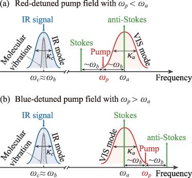
Figure 3. (a) and (b) Schematic diagram illustrating the upconversion of the IR signal to the VIS range within a molecular optomechanical system under the red-detuned and blue-detuned pump fields. It should be noted that the IR signal is treated as part of the input $c_{\mathrm{in}}$ of cavity IR mode. |
Under the above RWA conditions, the fast-oscillating terms $(\mathcal{G}_{a}\delta a^{\dagger}\delta B^{\dagger}+\mathrm{H.c.})$ and $(G_{c}\delta B^{\dagger}\delta c^{\dagger}+\mathrm{H.c.})$ in equation (6 ) can be neglected. The linearized QLEs in equation (5 ) is obtained as, 23 ) is written as 8 ), and the damping matrix $\mathcal{J}$ is given by $\mathcal{\mathcal{J}} = \mathrm{diag}(\sqrt{2\kappa_{a}},\sqrt{2\kappa_{c}},\sqrt{2\gamma_{B}})$.
$\begin{align} \delta\dot{a} & = -\left({\mathrm{i}}\Delta+\kappa_{a}\right)\delta a-{\mathrm{i}}\mathcal{G}_{a}\delta B+\sqrt{2\kappa_{a}}a_{\mathrm{in}},\nonumber\\ \delta\dot{c} & = -\left({\mathrm{i}}\omega_{c}+\kappa_{c}\right)\delta c-{\mathrm{i}}G_{c}\delta B+\sqrt{2\kappa_{c}}c_{\mathrm{in}},\nonumber\\ \delta\dot{B} & = -\left({\mathrm{i}}\omega_{b}+\gamma_{B}\right)\delta B-{\mathrm{i}}\mathcal{G}_{a}^{*}\delta a-{\mathrm{i}}G_{c}\delta c+\sqrt{2\gamma_{B}}B_{\mathrm{in}}.\end{align}$
By defining the fluctuation vector $\mathcal{V} = (\delta a,\delta c,\delta B)^{\mathrm{T}}$ and the input field vector $\mathcal{V}_{\mathrm{in}} = (a_{\mathrm{in}},c_{\mathrm{in}},B_{\mathrm{in}})^{\mathrm{T}}$, the linearized QLEs ($\begin{align} \frac{{\mathrm{d}}\mathcal{V}}{{\mathrm{d}}t} = -P\mathcal{V}+\mathcal{J}\mathcal{V}_{\mathrm{in}},\end{align}$
where the coefficient matrix $P$ is given in equation (In the case of only the IR signal in the input, the output spectrum of the VIS mode in the frequency domain is given by
$\begin{align} S_{a,\mathrm{out}}\left(\omega\right) = \mathcal{T}_{ac}^{\,{\mathrm{rd}}}\left(\omega\right)\left[S_{c,\mathrm{in}}\left(\omega\right)+\frac{1}{2}\right]+S_{a,\mathrm{add}}\left(\omega\right),\end{align}$
where the conversion efficiency $\mathcal{T}_{ac}^{\,{\mathrm{rd}}}(\omega)$ from the IR signal to the VIS range is expressed as $\begin{align} \mathcal{T}_{ac}^{\,{\mathrm{rd}}}\left(\omega\right) & = \left|\mathcal{U}_{12}^{\mathrm{rd}}\left(\omega\right)\right|^{2}.\end{align}$
The added noise spectrum is given by $S_{a,\mathrm{add}}(\omega) = \left[\mathcal{T}_{aa}^{\mathrm{rd}}(\omega)+\mathcal{T}_{aB}^{\mathrm{rd}}(\omega)\right]/2$, where $\mathcal{T}_{aa}^{\mathrm{rd}}(\omega) = \left|\mathcal{U}_{11}^{\mathrm{rd}}(\omega)\right|^{2}$ and $\mathcal{T}_{aB}^{\mathrm{rd}}(\omega) = \left|\mathcal{U}_{13}^{\mathrm{rd}}(\omega)\right|^{2}.$ Here, $\mathcal{U}_{1j}^{\mathrm{rd}}(\omega)$ denotes the element in the first row and $j$th column of the scattering matrix $\mathcal{U}^{\mathrm{rd}}(\omega) = \mathcal{\mathcal{J}}(P+{\mathrm{i}}\omega I_{3})^{-1}\mathcal{\mathcal{J}}-I_{3}$, with $\mathcal{U}_{12}^{\mathrm{rd}}(\omega) = -2G_{c}\mathcal{G}_{a}\sqrt{\kappa_{a}\kappa_{c}}/\{G_{c}^{2}({\mathrm{i}}\Delta+{\mathrm{i}}\omega+\kappa_{a})+[\left|\mathcal{G}_{a}\right|^{2}+({\mathrm{i}}\Delta+{\mathrm{i}}\omega+\kappa_{a})({\mathrm{i}}\omega_{b}+{\mathrm{i}}\omega+\gamma_{B})]({\mathrm{i}}\omega_{c}+{\mathrm{i}}\omega+\kappa_{c})\}$.As shown in figure 3(a), we consider the red-detuned pump field with $\Delta = \omega_{b}$ and the resonance case with $\omega_{c} = \omega_{b}$. At the first anti-Stokes sideband of the pump field, i.e. $\omega_{p}+\omega_{b}$, the conversion efficiency from the IR signal to the VIS range is given by
$\begin{align} \mathcal{T}_{ac}^{\mathrm{rd},AS}\equiv\mathcal{T}_{ac}^{\,{\mathrm{rd}}}\left(\omega = -\omega_{b}\right) = \left|\frac{-2G_{c}\mathcal{G}_{a}\sqrt{\kappa_{a}\kappa_{c}}}{G_{c}^{2}\kappa_{a}+\left|\mathcal{G}_{a}\right|^{2}\kappa_{c}+\kappa_{a}\kappa_{c}\gamma_{B}}\right|^{2}.\end{align}$
When $\kappa_{a}\kappa_{c}\gamma_{B}\ll\{\left|\mathcal{G}_{a}\right|^{2}\kappa_{c},G_{c}^{2}\kappa_{a}\}$, the conversion efficiency $\mathcal{T}_{ac}^{\mathrm{rd},AS}$ approaches 1 under the condition $\left|\mathcal{G}_{a}\right|^{2}\kappa_{c}\simeq G_{c}^{2}\kappa_{a}$.At the first Stokes sideband of the pump field, i.e. $\omega_{p}-\omega_{b}$, the conversion efficiency from the IR signal to the VIS range is
$\begin{align} \mathcal{T}_{ac}^{\mathrm{rd},S}\equiv\mathcal{T}_{ac}^{\,{\mathrm{rd}}}\left(\omega = \omega_{b}\right) = \left|\frac{-2G_{c}\mathcal{G}_{a}\sqrt{\kappa_{a}\kappa_{c}}}{G_{c}^{2}\Gamma_{a}+\left|\mathcal{G}_{a}\right|^{2}\Gamma_{c}+\Gamma_{a}\Gamma_{c}\Gamma_{B}}\right|^{2},\end{align}$
where $\Gamma_{a} = 2{\mathrm{i}}\omega_{b}+\kappa_{a}$, $\Gamma_{c} = 2{\mathrm{i}}\omega_{b}+\kappa_{c}$, and $\Gamma_{B} = 2{\mathrm{i}}\omega_{b}+\gamma_{B}$.4. Blue-detuned pump field
We analyzed the conversion efficiency from the IR signal to the VIS range under the red-detuned pump field condition. In this section, we will extend the discussion to the conversion efficiency for a blue-detuned pump field (see figure 3(b)). Under the RWA conditions $\left\{\left|\mathcal{G}_{a}\right|,G_{c}\right\} \ll-\Delta\sim\omega_{b}\sim\omega_{c}$, the fast-oscillating terms $(\mathcal{G}_{a}\delta a^{\dagger}\delta B+\mathrm{H.c.})$ and $(G_{c}\delta B^{\dagger}\delta c^{\dagger}+\mathrm{H.c.})$ in equation (6 ) is usually considered to be negligible. Hence, we obtain the linearized QLEs as 29 ) is written as
$\begin{align} \delta\dot{a} & = -\left({\text{i}}\Delta+\kappa_{a}\right)\delta a-{\text{i}}\mathcal{G}_{a}\delta B^{\dagger}+\sqrt{2\kappa_{a}}a_{\text{in}},\nonumber \\ \delta\dot{c}^{\dagger} & = -\left(-{\text{i}}\omega_{c}+\kappa_{c}\right)\delta c^{\dagger}+{\text{i}}G_{c}\delta B^{\dagger}+\sqrt{2\kappa_{c}}c_{\text{in}}^{\dagger},\nonumber \\ \delta\dot{B}^{\dagger} & = -\left(-{\text{i}}\omega_{b}+\gamma_{B}\right)\delta B^{\dagger}+{\text{i}}\mathcal{G}_{a}^{*}\delta a+{\text{i}}G_{c}\delta c^{\dagger}+\sqrt{2\gamma_{B}}B_{\text{in}}^{\dagger}.\end{align}$
By defining the fluctuation vector $\mathcal{W} = (\delta a,\delta c^{\dagger},\delta B^{\dagger})^{\mathrm{T}}$ and the input field vector $\mathcal{W}_{\mathrm{in}} = (a_{\mathrm{in}},c_{\mathrm{in}}^{\dagger},B_{\mathrm{in}}^{\dagger})^{\mathrm{T}}$, the linearized QLEs ($\begin{align} \frac{{\mathrm{d}}\mathcal{W}}{{\mathrm{d}}t} = -\mathcal{M}\mathcal{W}+\mathcal{J}\mathcal{W}_{\mathrm{in}},\end{align}$
with the coefficient matrix$\begin{align} \mathcal{\mathcal{M}} = \left(\begin{array}{ccc} {\mathrm{i}}\Delta+\kappa_{a} & 0 &{\mathrm{i}}\mathcal{G}_{a}\\ 0 & -{\mathrm{i}}\omega_{c}+\kappa_{c} & -{\mathrm{i}}G_{c}\\ -{\mathrm{i}}\mathcal{G}_{a}^{*} & -{\mathrm{i}}G_{c} & -{\mathrm{i}}\omega_{b}+\gamma_{B} \end{array}\right).\end{align}$
With the input-output relation, the output spectrum of the VIS mode in the frequency domain is given by $\begin{align} S_{a,\mathrm{out}}\left(\omega\right) = \mathcal{\mathcal{T}}_{ac}^{\mathrm{bd}}\left(\omega\right)\left[S_{c,\mathrm{in}}\left(\omega\right)+\frac{1}{2}\right]+S_{a,\mathrm{add}}\left(\omega\right),\end{align}$
where the conversion efficiency $\mathcal{\mathcal{T}}_{ac}^{\mathrm{bd}}\left(\omega\right)$ from the IR signal to the VIS range is $\begin{align} \mathcal{\mathcal{T}}_{ac}^{\mathrm{bd}}\left(\omega\right) & = \left|\mathcal{U}_{12}^{\mathrm{bd}}\left(\omega\right)\right|^{2}.\end{align}$
The added noise spectrum is $S_{a,\mathrm{add}}(\omega) = \left[\mathcal{T}_{aa}^{\mathrm{bd}}(\omega)+\mathcal{T}_{aB}^{\mathrm{bd}}(\omega)\right]$ $/2$, where $\mathcal{\mathcal{T}}_{aa}^{\mathrm{bd}}\left(\omega\right) = \left|\mathcal{U}_{11}^{\mathrm{bd}}(\omega)\right|^{2}$ and $\mathcal{\mathcal{T}}_{aB}^{\mathrm{bd}}\left(\omega\right) = \left|\mathcal{U}_{13}^{\mathrm{bd}}(\omega)\right|^{2}$. Here, $\mathcal{U}_{1j}^{\mathrm{bd}}(\omega)$ is the element in the first row and $j$th column of the scattering matrix $\mathcal{\mathcal{U}}^{\mathrm{bd}}(\omega) = \mathcal{\mathcal{J}}(\mathcal{M}+{\mathrm{i}}\omega I_{3})^{-1}\mathcal{\mathcal{J}}-I_{3}$, and its specific component $\mathcal{U}_{12}^{\mathrm{bd}}(\omega)$ is expressed as $\mathcal{U}_{12}^{\mathrm{bd}}(\omega) = 2G_{c}\mathcal{G}_{a}\sqrt{\kappa_{a}\kappa_{c}}/\{G_{c}^{2}({\mathrm{i}}\Delta+{\mathrm{i}}\omega+\kappa_{a})+[({\mathrm{i}}\Delta+{\mathrm{i}}\omega+\kappa_{a})({\mathrm{i}}\omega-{\mathrm{i}}\omega_{b}+\gamma_{B})-\left|\mathcal{G}_{a}\right|^{2}]({\mathrm{i}}\omega-{\mathrm{i}}\omega_{c}+\kappa_{c})\}$.In figure 3(b), we consider the blue-detuned pump field with $\Delta = -\omega_{b}$ and the resonance case with $\omega_{c} = \omega_{b}$. At the first anti-Stokes sideband of the pump field, i.e. $\omega_{p}+\omega_{b}$, the conversion efficiency from the IR signal to the VIS range is given by 28 ). At the first Stokes sideband of the pump field, i.e. $\omega_{p}-\omega_{b}$, the conversion efficiency of the IR-to-VIS signal is
$\begin{align} \mathcal{\mathcal{T}}_{ac}^{\mathrm{bd},AS}\equiv\mathcal{T}_{ac}^{\mathrm{bd}}\left(\omega = -\omega_{b}\right) = \left|\frac{2G_{c}\mathcal{G}_{a}\sqrt{\kappa_{a}\kappa_{c}}}{G_{c}^{2}\Gamma_{a}-\left|\mathcal{G}_{a}\right|^{2}\Gamma_{c}+\Gamma_{a}\Gamma_{c}\Gamma_{B}}\right|^{2},\end{align}$
where $\Gamma_{o}$ (for $o = a,c,B$) is defined below equation ($\begin{align} \mathcal{\mathcal{T}}_{ac}^{\mathrm{bd},S}\equiv\mathcal{T}_{ac}^{\mathrm{bd}}\left(\omega = \omega_{b}\right) = \left|\frac{2G_{c}\mathcal{G}_{a}\sqrt{\kappa_{a}\kappa_{c}}}{G_{c}^{2}\kappa_{a}+\kappa_{a}\kappa_{c}\gamma_{B}-\left|\mathcal{G}_{a}\right|^{2}\kappa_{c}}\right|^{2}.\end{align}$
By analyzing equation (5. Results
Before discussing the impact of the added noise, we validate the RWA and present in figure 4 the conversion efficiency for IR-to-VIS signal upconversion. Figures 4(a) and (b) show the conversion efficiencies $T_{ac}^{l}(\omega)$ and $\mathcal{T}_{ac}^{l}(\omega)$ ($l = \mathrm{rd},\mathrm{bd}$) as functions of the frequency $\omega$ for the red-detuned ($\Delta = \omega_{b}$) and blue-detuned ($\Delta = -\omega_{b}$) pump fields, respectively. Here $T_{ac}^{\,{\mathrm{rd}}}(\omega)$ [$T_{ac}^{\mathrm{bd}}(\omega)$] denotes the specific case of $T_{ac}(\omega)$ in equation (18b ) corresponding to $\Delta = \omega_{b}$ ($\Delta = -\omega_{b}$). The solid lines represent the numerical results of $T_{ac}^{l}\left(\omega\right)$ without using the RWA, while the dash-dotted and dashed lines denote the analytical results of $\mathcal{T}_{ac}^{l}\left(\omega\right)$ under the RWA, with $\mathcal{T}_{ac}^{l}\left(\omega\right)$ given by equations (26 ) and (33 ), respectively. The results show that, under the present parameters, the conversion efficiencies $\mathcal{T}_{ac}^{l}$ and $T_{ac}^{l}$ are not in complete agreement. In particular, the significant deviations occur at the first Stokes (anti-Stokes) sideband of the red-detuned (blue-detuned) pump field. However, within the frequency range of interest, i.e. the range of the first anti-Stokes (Stokes) of the red-detuned (blue-detuned) pump field, the two conversion efficiencies agree qualitatively. For the blue-detuned pump field, the conversion efficiency exceeds 1 at both the first Stokes and anti-Stokes sidebands, indicating amplification of IR-to-VIS signal upconversion.
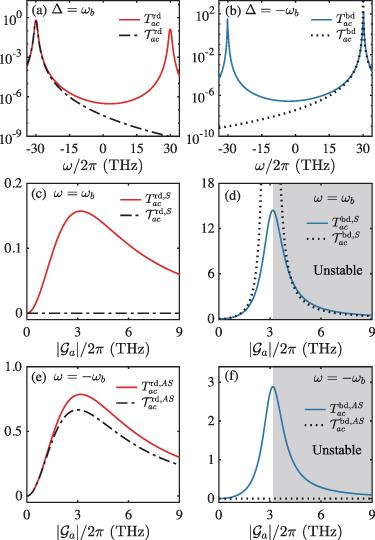
Figure 4. (a) and (b) Conversion efficiencies $T_{ac}^{l}\left(\omega\right)$ and $\mathcal{T}_{ac}^{l}\left(\omega\right)$ ($l = \mathrm{rd},\mathrm{bd}$, denoting the cases of red-detuned and blue-detuned pump fields, respectively) as functions of the frequency $\omega$ at $\left|\mathcal{G}_{a}\right|/2\pi = 3\,\mathrm{THz}$. (c) and (d) Conversion efficiencies $T_{ac}^{l,S}$ and $\mathcal{T}_{ac}^{l,S}$ at the first Stokes sideband ($\omega = \omega_{b}$) as functions of the coupling strength $\left|\mathcal{G}_{a}\right|$. (e) and (f) Conversion efficiencies $T_{ac}^{l,AS}$ and $\mathcal{T}_{ac}^{l,AS}$ at the first anti-Stokes sideband ($\omega = -\omega_{b}$) as functions of the coupling strength $\left|\mathcal{G}_{a}\right|$. In panels (a), (c), (e) (panels (b), (d), (f)), we use the red-detuned case of $\Delta = \omega_{b}$ (the blue-detuned case of $\Delta = -\omega_{b}$). Here we consider the resonance case with $\omega_{c} = \omega_{b} = 2\pi\times30\,\mathrm{THz}$, and other parameters are $N = 10^{7}$, $g_{c}/2\pi = 0.1\,\mathrm{GHz}$, $\varepsilon_{p}/2\pi = 500\,\mathrm{THz}$, $\kappa_{a}/2\pi = 30\,\mathrm{THz}$, $\kappa_{c}/2\pi = 0.5\,\mathrm{THz}$, and $\gamma_{B}/2\pi = 0.1\,\mathrm{THz}$. The gray shaded areas in panels (d) and (f) indicate the regions of instability (without applying the RWA). |
Figures 4(c) and (d) further show the conversion efficiencies $T_{ac}^{l,S} = T_{ac}^{l}(\omega = \omega_{b})$ and $\mathcal{T}_{ac}^{l,S}$ ($l = \mathrm{rd},\mathrm{bd}$) at the first Stokes sideband as functions of the coupling strength $\left|\mathcal{G}_{a}\right|$ for $\Delta = \omega_{b}$ and $\Delta = -\omega_{b}$, respectively. It is shown that, $T_{ac}^{l,S}$ initially increases with $\left|\mathcal{G}_{a}\right|$, reaches a maximum value (e.g. $T_{ac}^{\,{\mathrm{rd},S,\mathrm{max}}}\approx0.13$ and $T_{ac}^{\,{\mathrm{bd},S,\mathrm{max}}}\approx12$) at optimal coupling strength $\left|\mathcal{G}_{a}\right|\simeq2\pi\times3.48\,\mathrm{THz}$, and then decreases. Similarly, figures 4(e) and (f) display the conversion efficiencies $T_{ac}^{l,AS} = T_{ac}^{l}(\omega = -\omega_{b})$ and $\mathcal{T}_{ac}^{l,AS}$ at the first anti-Stokes sideband versus $\left|\mathcal{G}_{a}\right|$ for $\Delta = \omega_{b}$ and $\Delta = -\omega_{b}$, respectively. Here, $T_{ac}^{l,AS}$ reaches its maximum value (e.g. $T_{ac}^{\mathrm{rd},AS,\mathrm{max}}\approx0.66$ and $T_{ac}^{\mathrm{bd},AS,\mathrm{max}}\approx2.39$) at optimal coupling strength $\left|\mathcal{G}_{a}\right|\simeq2\pi\times3.48\,\mathrm{THz}$. Notably, under the red-detuned condition $\Delta = \omega_{b}$, the anti-Stokes sideband exhibits a higher conversion efficiency than the Stokes sideband, whereas the opposite behavior occurs under the blue-detuned condition $\Delta = -\omega_{b}$. At the first anti-Stokes (Stokes) sideband under the red- (blue-) detuned condition, the conversion efficiencies $\mathcal{T}_{ac}$ and $T_{ac}$ begin to deviate for the coupling strength $\left|\mathcal{G}_{a}\right|\gtrsim2\pi\times1\,\mathrm{THz}$, as shown in figures 4(d) and (e). Nevertheless, the qualitative physical picture remains consistent, especially regarding the resonance peak positions. Based on these findings, we next analyze the conversion efficiency and the added noise without applying the RWA.
We now discuss the impact of the added noise. Figures 5(a) and (c) show the conversion efficiency $T_{ac}^{\,{\mathrm{rd}}}(\omega)$ and the added noise $n_{\mathrm{add}}^{AS}(\omega)$ at the first anti-Stokes sideband as functions of the frequency $\omega$, under the red-detuned condition $\Delta = \omega_{b}$ for different coupling strengths $\left|\mathcal{G}_{a}\right|$. As shown in figures 5(a) and (c), the peak value of the conversion efficiency increases with $\left|\mathcal{G}_{a}\right|$, while the added noise decreases. Notably, at large $\left|\mathcal{G}_{a}\right|$, the added noise on resonance ($\omega = -\omega_{b}$) approaches half a quantum, i.e. $n_{\mathrm{add}}^{AS}\rightarrow1/2$. In contrast, figures 5(b) and (d) present the conversion efficiency $T_{ac}^{\mathrm{bd}}(\omega)$ and the added noise $n_{\mathrm{add}}^{S}(\omega)$ at the first Stokes sideband under the blue-detuned condition $\Delta = -\omega_{b}$ for $\left|\mathcal{G}_{a}\right|/2\pi = 1,2,3\,\mathrm{THz}$. With increasing coupling strength $\left|\mathcal{G}_{a}\right|$, the conversion efficiency increases with $\left|\mathcal{G}_{a}\right|$, whereas the added noise exhibits a non-monotonic behavior. At $\left|\mathcal{G}_{a}\right|/2\pi = 2\,\mathrm{THz}$, the added noise on resonance ($\omega = \omega_{b})$ reaches 1.3.
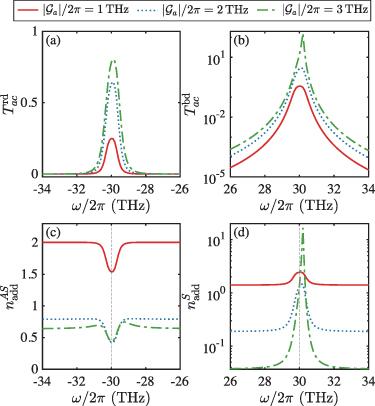
Figure 5. (a), (c) Conversion efficiency $T_{ac}^{\,{\mathrm{rd}}}(\omega)$ and added noise $n_{\mathrm{add}}^{AS}(\omega)$ at the first anti-Stokes sideband, and (b), (d) conversion efficiency $T_{ac}^{\mathrm{bd}}(\omega)$ and added noise $n_{\mathrm{add}}^{S}(\omega)$ at the first Stokes sideband, as functions of the frequency $\omega$. The results correspond to the red-detuned ($\Delta = \omega_{b}$) and blue-detuned ($\Delta = -\omega_{b}$) cases, respectively, with coupling strength $\left|\mathcal{G}_{a}\right|/2\pi = 1,2,3\,\mathrm{THz}$. Here we consider the resonance case of $\omega_{c} = \omega_{b} = 2\pi\times30\,\mathrm{THz}$, and other parameters are the same as those in figure 4. |
We further analyze how the system parameters-$\left|\mathcal{G}_{a}\right|$ and $\kappa_{a}$-affect both the conversion efficiency and added noise. Figures 6(a) and (c) show the conversion efficiency $T_{ac}^{\mathrm{rd},AS}$ (dotted curves) and the added noise $n_{\mathrm{add}}^{AS}$ on resonance (solid curves) at the first anti-Stokes sideband under the red-detuned condition $\Delta = \omega_{b}$. As illustrated in figures 6(a) and (c), the conversion efficiency first increases and then decreases with $\left|\mathcal{G}_{a}\right|$ and $\kappa_{a}$, while the added noise shows the reverse trend. By tuning the coupling strength and decay rate of the system, the added noise can be suppressed to a level below half a quantum; however, the conversion efficiency $T_{ac}^{\mathrm{rd},AS}\lesssim1$. In figures 6(b) and (d), we show the conversion efficiency $T_{ac}^{\,{\mathrm{bd},S}}$ (dotted curves) and the added noise $n_{\mathrm{add}}^{S}$ on resonance (solid curves) at the first Stokes sideband under the blue-detuned condition $\Delta = -\omega_{b}$. In the stable regime, the conversion efficiency increases with $\left|\mathcal{G}_{a}\right|$ but decreases with $\kappa_{a}$, while the added noise shows the reverse trend. In addition, at $\left|\mathcal{G}_{a}\right| = 2\pi\times0.75\,\mathrm{THz}$ and $\kappa_{a}/2\pi = 2\,\mathrm{THz}$, we find that the conversion efficiency reaches $T_{ac}^{\,{\mathrm{bd},S}}\approx10^{3}$, while the added noise approaches the quantum limit of one quantum, i.e. $n_{\mathrm{add}}^{S}\rightarrow1$. This implies that the added noise of the system can be reduced to the fundamental limit caused by unavoidable vacuum fluctuations. Compared with the red-detuned case, the added noise increases by 2 to 3 times, while the conversion efficiency is amplified by three orders of magnitude.
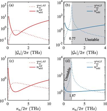
Figure 6. Conversion efficiency $T_{ac}^{\mathrm{rd},AS}$ and added noise $n_{\mathrm{add}}^{AS}$ on resonance at the first anti-Stokes sideband as functions of (a) $\left|\mathcal{G}_{a}\right|$ for $\kappa_{a}/2\pi = 2\,\mathrm{THz}$ and (c) $\kappa_{a}$ for $\left|\mathcal{G}_{a}\right|/2\pi = 0.75\,\mathrm{THz}$ under the red-detuned condition $\Delta = \omega_{b}$. Conversion efficiency $T_{ac}^{\,{\mathrm{bd},S}}$ and added noise $n_{\mathrm{add}}^{S}$ on resonance at the first Stokes sideband as functions of (b) $\left|\mathcal{G}_{a}\right|$ for $\kappa_{a}/2\pi = 2\,\mathrm{THz}$ and (d) $\kappa_{a}$ for $\left|\mathcal{G}_{a}\right|/2\pi = 0.75\,\mathrm{THz}$ under the blue-detuned condition $\Delta = -\omega_{b}$. Other parameters are the same as those in figure 4. |
So far, the analysis of the IR-to-VIS signal conversion efficiency has focused on the resonant case, where the frequencies of the IR mode and molecular vibrational mode are perfectly matched. However, in realistic experiments, exact resonance is not always achieved. In the following, we investigate the IR-to-VIS conversion efficiency under near-resonant conditions. In figure 7(a), we show the conversion efficiency $T_{ac}^{\mathrm{rd},AS}$ at the first anti-Stokes sideband as a function of $\left|\mathcal{G}_{a}\right|$ for different values of $\omega_{c}$ under the red-detuned condition $\Delta = \omega_{b}$. Here, we define the detuning as $\delta = \omega_{c}-\omega_{b}$. The results show that, for a fixed $\left|\mathcal{G}_{a}\right|$, the conversion efficiency $T_{ac}^{\mathrm{rd},AS}$ decreases as $|\delta|$ increases. In figure 7(b), we plot the conversion efficiency $T_{ac}^{\,{\mathrm{bd},S}}$ at the first Stokes sideband as a function of $\left|\mathcal{G}_{a}\right|$ for different values of $\omega_{c}$ under the blue-detuned condition $\Delta = -\omega_{b}$. The unstable regions vary under different parameter sets and are therefore not explicitly marked here. It can be seen that $T_{ac}^{\,{\mathrm{bd},S}}$ may exceed 1 under near-resonant conditions. In contrast to the red-detuned case, the conversion efficiency $T_{ac}^{\,{\mathrm{bd},S}}$ under non-resonant conditions (e.g. $\omega_{c}/2\pi = 31\,\text{THz}$) can even surpass that obtained under exact resonance.
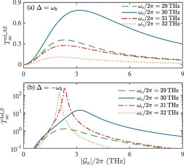
Figure 7. (a) Conversion efficiency $T_{ac}^{\mathrm{rd},AS}$ at the first anti-Stokes sideband as a function of $\left|\mathcal{G}_{a}\right|$ for different values of $\omega_{c}$ under the red-detuned condition $\Delta = \omega_{b}$. (b) Conversion efficiency $T_{ac}^{\,{\mathrm{bd},S}}$ at the first Stokes sideband as a function of $\left|\mathcal{G}_{a}\right|$ for different values of $\omega_{c}$ under the blue-detuned condition $\Delta = -\omega_{b}$. Other parameters are the same as those in figure 4. |
It is worth noting that current experimental implementations of molecular optomechanical systems typically involve only several hundred molecules. To evaluate the conversion efficiency under more realistic conditions, figure 8 presents the IR-to-VIS conversion efficiency obtained using experimentally feasible parameters [11-13, 51]. The results exhibit the same overall behavior as those shown in figures 4(d) and (e). In particular, the amplification of IR signal can still be achieved within an appropriate parameter regime under the blue-detuned condition.
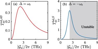


Figure 8. (a) Conversion efficiency $T_{ac}^{\mathrm{rd},AS}$ at the first anti-Stokes sideband as a function of $\left|\mathcal{G}_{a}\right|$ under the red-detuned condition $\Delta = \omega_{b}$. (b) Conversion efficiency $T_{ac}^{\,{\mathrm{bd},S}}$ at the first Stokes sideband as a function of $\left|\mathcal{G}_{a}\right|$ under the blue-detuned condition $\Delta = -\omega_{b}$. Other parameters are $\omega_{c}/2\pi = 32\,\mathrm{THz}$, $\omega_{b}/2\pi = 32.4\,\mathrm{THz}$, $N = 365$, $g_{c}/2\pi = 10\,\mathrm{GHz}$, $\varepsilon_{p}/2\pi = 500\,\mathrm{THz}$, $\kappa_{a}/2\pi = 30\,\mathrm{THz}$, $\kappa_{c}/2\pi = 0.5\,\mathrm{THz}$, and $\gamma_{B}/2\pi = 0.1\,\mathrm{THz}$. The gray shaded area in panel (b) indicates the unstable region. |
6. Conclusion
In conclusion, we have calculated the conversion efficiency from IR signal to VIS range and the noise added to the upconverted signal in a molecular optomechanical cavity, where the molecular vibrations are coupled to both the IR and VIS modes. Our results indicate that, under the red-detuned condition, the conversion efficiency of the anti-Stokes sideband is higher than that of the Stokes sideband, whereas the conversion efficiency of the Stokes sideband surpasses that of the anti-Stokes sideband under the blue-detuned condition, where amplification of the IR signal is achieved. In addition, we find that the added noise remains below half a quantum under the red-detuned condition, while it approaches the quantum limit of one quantum under the blue-detuned condition. Compared with the red-detuned regime, the added noise in the blue-detuned regime increases by a factor of 2 to 3, while the conversion efficiency is amplified by three orders of magnitude. Our research seeks to establish a theoretical basis to support experimental progress in IR signal upconversion.