

1. Introduction
Ultracold molecules provide a versatile platform for advancing quantum science, spanning ultracold chemistry [1-6], precision metrology [7-10], quantum computation [11-14] and quantum simulation [4, 14-16]. In particular, polar molecules possess permanent electric dipole moments that give rise to strong, long-range dipole-dipole interactions. These interactions can be controlled by engineering the rich internal structure with external fields [17-19], offering new opportunities to explore many-body physics and strongly correlated quantum phenomena in previously inaccessible regimes [19-26].
However, polar molecules suffer short-range collision losses, which makes it challenging to stabilize samples of ultracold molecules [27-30]. Shielding techniques offer an effective route to suppress such detrimental losses by engineering a repulsive potential that prevents molecules from reaching the short-range loss region. In two-dimensional (2D) systems, a strong static electric field (E-field) applied perpendicular to the plane induces repulsive side-by-side dipolar interactions between polarized molecules, realizing effective 2D shielding [31]. For three-dimensional (3D) systems, however, shielding with a static E-field requires resonant dipolar coupling within a narrow field-strength window [32-35]. Alternatively, a blue-detuned circularly polarized microwave field can realize a fully 3D repulsive short-range potential, which effectively suppresses collision losses [36-45] and has enabled the creation of quantum-degenerate Fermi gases of polar molecules [39]. Recently, a Bose-Einstein condensate of polar bosonic molecules has been realized using double microwave dressing that combines linearly and circularly polarized fields [44]. This approach compensates for the attractive dipole-dipole interactions at long range while preserving the short-range repulsive barrier.
The effective inter-molecule interaction generated by either a static E-field or a microwave dressing alone [46-50], as well as the corresponding adiabatic mutual gauge field [50], has been extensively studied. Additionally, Ref. [51], investigates the effective potential in different shielding schemes including the combined use of a static E-field and a circularly polarized microwave, with the single-molecule Hilbert space restricted to four lowest rotational states with J = 0 and J = 1. For sufficiently strong static E-field, however, even higher rotational states are significantly admixed and must be included. On the other hand, the adiabatic mutual gauge field, which is associated with the combination of a static E-field and a microwave, has not been studied.
In this work, we investigate the effective pairwise interaction and adiabatic mutual gauge field of ultracold molecules dressed by both a circularly polarized microwave and a strong static electric field (figure 1), considering all rotational states that are significantly coupled by the static field. We demonstrate that the static electric field strength Ez can be divided into three distinct regions, separated by two critical values, ${E}_{c}^{(1)}$ and ${E}_{c}^{(2)}$ (${E}_{c}^{(2)}\gt {E}_{c}^{(1)}$). The behavior of the effective interaction in these regions varies qualitatively. In particular, the repulsive shielding vanishes when ${E}_{z}\gt {E}_{c}^{(2)}$. Furthermore, the mutual gauge field is highly tunable via the static electric field. Our findings provide valuable insights for manipulating ultracold molecules in future experiments.
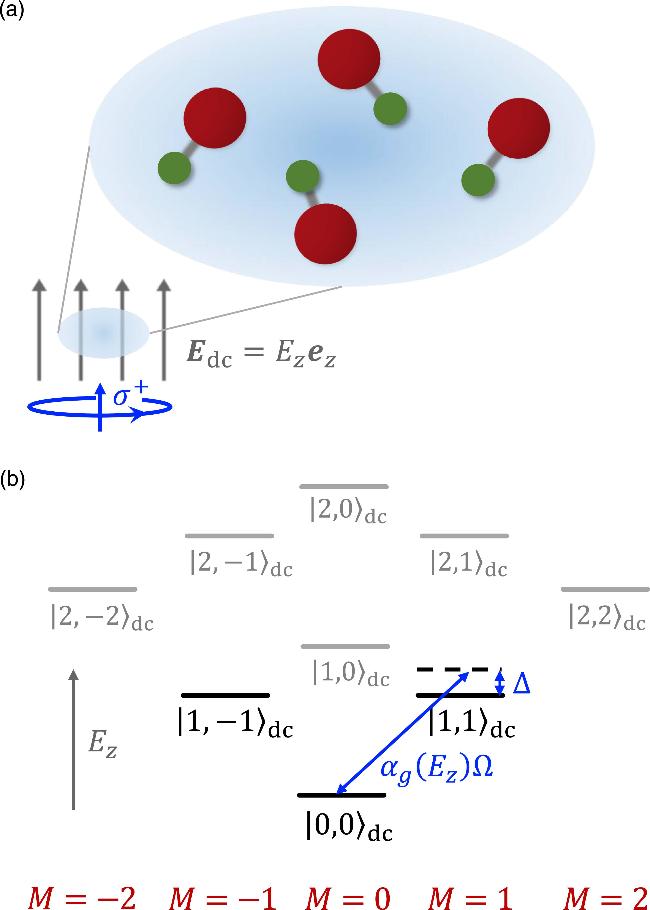
Figure 1. (a) Schematic diagram of molecules simultaneously dressed by a static electric field and a σ+-polarized microwave field, both applied along the z axis. The z axis defines the quantization direction. (b) Schematic diagrams of the dc Stack level for a single molecule. The {|0, 0$\rangle$dc, |1, 1$\rangle$dc} manifold constitutes the effective single-molecule model. |0, 0$\rangle$dc and |1, 1$\rangle$dc are coupled by circular polarized microwave with Ez-dependent strength αg(Ez)Ω. When static E-field is absent, the coefficient αg(Ez = 0) = 1. |
The remainder of this paper is organized as follows: in section 2 we introduce our system and the model we use, including the single-molecule level structure, the dipole-dipole interaction, and the basis set used in our calculations. Section 3 presents the results for the effective potential and mutual synthetic gauge field. A summary of this work is given in section 4 .
2. System and model
We consider a gas of 1Σ+ polar molecules in the vibrational ground state v = 0. Neglecting hyperfine interactions, the molecular internal structure is described by rotational degrees of freedom. The molecules are simultaneously dressed by a static electric field and a σ+-polarized microwave field, as sketched in figure 1(a). The static E-field 2 ), (3 ), ${\rm{\Lambda }}{\hat{{\boldsymbol{J}}}}^{2}$ is the free Hamiltonian of the rotational states, and $-\hat{{\boldsymbol{d}}}\cdot {{\boldsymbol{E}}}_{{\rm{dc}}}$ and $-\hat{{\boldsymbol{d}}}\cdot {{\boldsymbol{E}}}_{+}(t)$ describes the coupling of the molecule with the static E-field and the microwave, respectively. For convenience, we denote |J, M$\rangle$dc (J = 0, 1, 2, . . . ;M = 0, 1, $\text { ± }$, J) as the eigen-states of ${\hat{H}}_{{\rm{dc}}}$ in the space with Jz = M, with corresponding eigen-energy EJ,|M|, where Jz is the molecular angular momentum along th z-direction of the lab frame. Here we choose the convention ${\left.| J,M{\rangle }_{{\rm{dc}}}\right|}_{{E}_{z}=0}=| J,M\rangle $, where |J, M$\rangle$ is the bare rotational states, i.e. the common eigen-states of ${\hat{{\boldsymbol{J}}}}^{2}$ and ${\hat{J}}_{z}$. Clearly, in the presence of the static E-field, |J, M$\rangle$dc is a superposition of states $| {J}^{{\prime} },M\rangle $ with different ${J}^{{\prime} }$, i.e.4 ), (5 ) for 0 ≤ J ≤ 9, which is accurate enough for the static E-field strength considered in this work [52].
$\begin{eqnarray}{{\boldsymbol{E}}}_{{\rm{dc}}}={E}_{z}{{\boldsymbol{e}}}_{z},\end{eqnarray}$
is applied along z direction, and the microwave field ${{\boldsymbol{E}}}_{+}(t)={E}_{+}[\cos (\omega t){{\boldsymbol{e}}}_{x}+\sin (\omega t){{\boldsymbol{e}}}_{y}]$ propagates along the z axis with σ+ polarization and frequency ω. The single-molecule Hamiltonian ${\hat{H}}_{0}$ is $\begin{eqnarray}{\hat{H}}_{0}={\hat{H}}_{{\rm{dc}}}-\hat{{\boldsymbol{d}}}\cdot {{\boldsymbol{E}}}_{+}(t),\end{eqnarray}$
where $\begin{eqnarray}{\hat{H}}_{{\rm{dc}}}={\rm{\Lambda }}{\hat{{\boldsymbol{J}}}}^{2}-\hat{{\boldsymbol{d}}}\cdot {{\boldsymbol{E}}}_{{\rm{dc}}}.\end{eqnarray}$
Here $\hat{{\boldsymbol{J}}}$ is the angular momentum operator associated with the rotation of the molecular axis, $\Lambda$ is the molecular rotational constant, and $\hat{{\boldsymbol{d}}}$ is the electric dipole operator of molecule. In equations ( $\begin{eqnarray}| J,M{\rangle }_{{\rm{dc}}}=\displaystyle \sum _{{J}^{{\prime} }=0}^{\infty }{c}_{J,{J}^{{\prime} }}^{M}({E}_{z})| {J}^{{\prime} },M\rangle .\end{eqnarray}$
Additionally, in the basis of {|J, M$\rangle$dc}, the Hamiltonian ${\hat{H}}_{{\rm{dc}}}$ can be expressed as $\begin{eqnarray}{\hat{H}}_{{\rm{dc}}}=\displaystyle \sum _{M=-\infty }^{\infty }\displaystyle \sum _{J=| M| }^{\infty }{E}_{J,| M| }| J,M{\rangle }_{{\rm{dc}}}\langle J,M| .\end{eqnarray}$
In our calculation, we perform the summation ∑J of equations (Owing to the intrinsic anharmonicity, and with accidental degeneracies excluded, the internal dynamics are well captured by the three lowest dressed states, which are donated as |g$\rangle$ ≡ |0, 0$\rangle$dc, |e1$\rangle$ ≡ |1, 1$\rangle$dc, and |e-1$\rangle$ ≡ |1, - 1$\rangle$dc. Note that within the parameter regime considered here, the |1, 0$\rangle$dc state is energetically far detuned from the lowest three states with respect to both their internal splitting E1,1 and the microwave frequency ω. As a result, no resonant transition connects the three-state subspace to |1, 0$\rangle$dc via either the microwave field or the dipole-dipole interaction. Since our goal is to shield molecules prepared in the ground state, the |1, 0$\rangle$dc state can therefore be safely excluded from the effective model. Figure 1(b) shows a schematic of the single-molecule model. Restricted to this three-state subspace, the single-particle Hamiltonian after applying the rotating-wave approximation (RWA) becomes A ) We assume the energy difference between |1, 0$\rangle$dc and |e1$\rangle$ is sufficiently detuned from ω so that the coupling between |1, 0$\rangle$dc and |e1$\rangle$ can be neglected in the present treatment. The dipole-dipole interaction between two polar molecules is A )
$\begin{eqnarray}{\hat{H}}_{0}=\displaystyle \sum _{i=\pm 1}{E}_{1}| {e}_{i}\rangle \langle {e}_{i}| +\frac{\hslash {\rm{\Omega }}}{2}\left[{\alpha }_{g}({E}_{z})| {e}_{1}\rangle \langle g| {{\rm{e}}}^{-{\rm{i}}\omega t}+{\rm{H.c.}}\right],\end{eqnarray}$
where E1 = E1,1 - E0,0 is the energy difference between |e$\rangle$ and |g$\rangle$, Ω is the zero-static E-field coupling strength, and the coefficient αg(Ez) reduces to unit in the absence of static E-field (see details in Appendix $\begin{eqnarray}{\hat{H}}_{{\rm{int}}}({\boldsymbol{r}})=\frac{1}{4\pi {\epsilon }_{0}{r}^{3}}\left[{\hat{{\boldsymbol{d}}}}_{1}\cdot {\hat{{\boldsymbol{d}}}}_{2}-3({\hat{{\boldsymbol{d}}}}_{1}\cdot \hat{{\boldsymbol{r}}})({\hat{{\boldsymbol{d}}}}_{2}\cdot \hat{{\boldsymbol{r}}})\right],\end{eqnarray}$
where r ≡ r1 - r2 is the relative position of the two molecules, ${\hat{{\boldsymbol{d}}}}_{j}$ is the electric dipole operator of the molecule j, and ε0 is the dielectric constant. The dipole-dipole interaction has a characteristic length defined as rd = md2/(12$\pi$ℏ2ε0), where m is the molecular mass and d being the dipole moment. For NaCs molecules, this length scale is rd = 3.3 × 10⁵a0, with a0 the Bohr radius. The associated energy scale is given by ${E}_{d}={\hslash }^{2}/(2m{r}_{d}^{2})$. Under the RWA, only the near-resonance interaction processes are retained, and the dipole-dipole interaction reduces to [46] $\begin{eqnarray}{\hat{V}}_{\,\rm{dd}\,}({\boldsymbol{r}})=\frac{{d}^{2}}{\sqrt{30\pi }{\epsilon }_{0}{r}^{3}}\displaystyle \sum _{m=0,\pm 2}\left[\right.{\hat{{\rm{\Sigma }}}}_{2,m}{{\rm{Y}}}_{2}^{m* }(\theta ,\phi )\left]\right.,\end{eqnarray}$
where θ and φ are the polar and the azimuthal angles of of r, respectively, and ${{\rm{Y}}}_{2}^{m}(\theta ,\phi )$ are the spherical harmonics. The operators ${\hat{{\rm{\Sigma }}}}_{2,m}$ take the form (detailed in Appendix $\begin{eqnarray}\begin{array}{rcl}{\hat{{\rm{\Sigma }}}}_{2,0} & = & \frac{1}{\sqrt{6}}\left[{\alpha }_{g}^{2}({E}_{z})\left(| {e}_{1};g\rangle \langle g;{e}_{1}| +| {e}_{-1};g\rangle \langle g;{e}_{-1}| \right.\right.\\ & & \left.\left.+\,\rm{H.c.}\,\right)-2{\hat{h}}_{0}\displaystyle \otimes {\hat{h}}_{0}\right],\end{array}\end{eqnarray}$
$\begin{eqnarray}\begin{array}{rcl}{\hat{{\rm{\Sigma }}}}_{2,2} & = & {\alpha }_{g}^{2}({E}_{z})\left(\right.| {e}_{1};g\rangle \langle g;{e}_{-1}| +| g;{e}_{1}\rangle \langle {e}_{-1};g| \left)\right.,\end{array}\end{eqnarray}$
$\begin{eqnarray}\begin{array}{rcl}{\hat{{\rm{\Sigma }}}}_{2,2} & = & {\hat{{\rm{\Sigma }}}}_{2,2}^{\dagger },\end{array}\end{eqnarray}$
where ${\hat{h}}_{0}={\beta }_{g}({E}_{z})| g\rangle \langle g| +{\beta }_{e}({E}_{z})\left(| {e}_{1}\rangle \langle {e}_{1}| +| {e}_{-1}\rangle \langle {e}_{-1}| \right)$. Throughout, we use the notation |s1;s2$\rangle$ ≡ |s1$\rangle$1|s2$\rangle$2(s1,2 = g, e1).In the time-independent rotating frame, the single-molecule Hamiltonian (6 ) takes the form 6 )-(9 ) in this rotating frame.
$\begin{eqnarray}{\hat{H}}_{0}={\rm{\Delta }}| g\rangle \langle g| +\frac{\hslash {\rm{\Omega }}}{2}\left[{\alpha }_{g}({E}_{z})| {e}_{1}\rangle \langle g| +{\rm{H.c.}}\right],\end{eqnarray}$
where Δ = ω - 2E1 > 0 corresponding to the blue detuning regime. Dipole-dipole interaction retains the structure of equations (For the two-molecules problems, the total Hamiltonian in the center-of-mass framework becomes
$\begin{eqnarray}\begin{array}{rcl}{H}_{{\rm{2b}}} & = & -\frac{{\hslash }^{2}}{2\mu }{{\rm{\nabla }}}^{2}+\hat{W}({\boldsymbol{r}}),\end{array}\end{eqnarray}$
$\begin{eqnarray}\begin{array}{rcl}\hat{W}({\boldsymbol{r}}) & = & \displaystyle \sum _{j=1,2}{\hat{H}}_{0}^{(j)}+{\hat{V}}_{\,\rm{dd}\,}({\boldsymbol{r}}),\end{array}\end{eqnarray}$
where μ = m/2 is the reduced mass of two molecules, and $\hat{W}({\boldsymbol{r}})$ represents the internal coupling between the two molecules, where the underlying dipole-dipole interaction is modified by the microwave dressing and the static E-field.3. Effective potential between two molecules
With the Born-Oppenheimer approximation, the adiabatic interaction potentials are obtained by diagonalizing $\hat{W}({\boldsymbol{r}})$. In the context of shielding, the effective potential V(r) is given by the highest eigenvalue of $\hat{W}({\boldsymbol{r}})$, while the internal state adiabatically follows the corresponding eigenstate |ζ(r)$\rangle$. With the total two-molecule wave function written in the center-of-mass frame as B )
$\begin{eqnarray}| {\rm{\Psi }}({\boldsymbol{r}})\rangle =\psi ({\boldsymbol{r}})| \zeta ({\boldsymbol{r}})\rangle ,\end{eqnarray}$
the relative-motion wave function ψ(r) obeys an effective Hamiltonian (see details in Appendix $\begin{eqnarray}\hat{{ \mathcal H }}=\frac{1}{2\mu }{\left[-{\rm{i}}\hslash {{\rm{\nabla }}}_{{\boldsymbol{r}}}-{\boldsymbol{A}}({\boldsymbol{r}})\right]}^{2}+V({\boldsymbol{r}}),\end{eqnarray}$
with the induced gauge field $\begin{eqnarray}{\boldsymbol{A}}({\boldsymbol{r}})={\rm{i}}\hslash \langle \zeta ({\boldsymbol{r}})| {{\rm{\nabla }}}_{{\boldsymbol{r}}}| \zeta ({\boldsymbol{r}})\rangle .\end{eqnarray}$
3.1. Shielding potential V(r)
For our system, V(r) ≡ V(r, θ) is independent of φ, due to the cylindrical symmetry of the static electric field and σ+ microwave field. In the presence of microwave shielding alone, the effective interaction between two polar molecules consists of a short-range repulsive core together with a long-range anti-dipolar potential that is repulsive along z axis and attractive in the transverse xy-plane [46]. A static E-field, by contrast, tends to polarize the molecules along its direction and produces the usual dipolar interaction. When both fields are applied, increasing the static E-field strength continuously reshapes the effective interaction, giving rise to three distinct regimes, separated by two critical strengths ${E}_{c}^{(1)}$ and ${E}_{c}^{(2)}$, as shown in figures 2(a)-(c) with a typical example, and introduced in detail in the following:
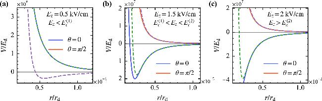
Figure 2. Effective interaction potentials V(r, θ) for two molecules at static E-field strengths in three distinct regimes: (a) Ez = 0.5 kV cm-1 (${E}_{z}\lt {E}_{c}^{(1)}$), (b) Ez = 1.5 kV cm-1 (${E}_{c}^{(1)}\lt {E}_{z}\lt {E}_{c}^{(2)}$), and (c) Ez = 2 kV cm-1 (${E}_{c}^{(1)}\lt {E}_{z}\lt {E}_{c}^{(2)}$). Solid lines show the exact diagonalization results for V(r, θ = 0) (blue) and V(r, θ = $\pi$/2) (orange) respectively. Dashed lines are perturbative results from equation ( |
3.1.1. ${E}_{z}\lt {E}_{c}^{(1)}$
For a weak static E-field with ${E}_{z}\lt {E}_{c}^{(1)}$, the long-range behavior of V(r) is 'anti-dipolar', i.e. is repulsive along the z-axis (θ = 0), and attractive in the x-y plane (θ = $\pi$/2). Moreover, in the short-range region, V(r) has a repulsive core in all the directions, as shown in figure 2(a). This behavior is similar to that obtained with microwave dressing alone [46]. Additionally, by treating ${\hat{V}}_{\,\rm{dd}\,}({\boldsymbol{r}})$ perturbatively up to second order, we can obtain an approximated expression for this effective potential: A . We further denote the zero crossing of V(r) in xy-plane by rc, which effectively defines a shielding radius, as the effective potential rises sharply and becomes repulsive in all directions for r < rc.
$\begin{eqnarray}{V}_{{\rm{pert}}}(r,\theta )=\frac{{C}_{3}}{{r}^{3}}(1-3{\cos }^{2}\theta )+\frac{{C}_{6}(\theta )}{{r}^{6}},\end{eqnarray}$
where C3 < 0 and C6(θ) > 0 depends on Ez and Ω/Δ, as detailed in Appendix Moreover, as shown in figures 3(a), (b), |C3| decreases and rc increases with the increasing of Ez. This yields that the long-range anti-dipole interaction and the short-range repulsive interaction become weaker and stronger as Ez increases, respectively. At the critical E-field ${E}_{z}={E}_{c}^{(1)}$ we have
$\begin{eqnarray}\begin{array}{r}{C}_{3}({E}_{c}^{(1)})=0,{r}_{c}({E}_{c}^{(1)})=\infty .\end{array}\end{eqnarray}$
Thus, at ${E}_{z}={E}_{c}^{(1)}$ the long-range anti-dipole interaction vanishes, and the effective inter-molecule potential is repulsive in all the directions.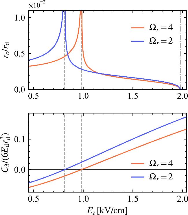
Figure 3. (a) The shielding radius rc and (b) the long-range coefficient in equation ( |
3.1.2. ${E}_{c}^{(1)}\lt {E}_{z}\lt {E}_{c}^{(2)}$
For an intermediate static E-field with ${E}_{c}^{(1)}\lt {E}_{z}\lt {E}_{c}^{(2)}$, which we refer to as the dipolar regime, the long-range effective interaction crosses over to a dipolar form, which is attractive along the z-axis (θ = 0), and repulsive in the x-y plane (θ = $\pi$/2). In addition, there is also a short-range repulsive core, as shown in figure 2(b). Consequently, the effective interaction potential can also be approximated via equation (18 ), while now we have C3 > 0 and rc > 0.
Furthermore, as shown in figure 3, C3 increases while rc decreases with Ez. Thus, the long-range dipolar interaction and the short-range repulsive interaction becomes stronger and weaker as the increasing of Ez, respectively. When the static E-field intensity Ez reaches to the second critical point ${E}_{c}^{(2)}$, we have
$\begin{eqnarray}\begin{array}{r}0\lt {C}_{3}({E}_{c}^{(2)})\lt \infty ,\,{r}_{c}({E}_{c}^{(2)})=0.\end{array}\end{eqnarray}$
Namely, the short-range repulsive core completely vanishes.3.1.3. ${E}_{z}\gt {E}_{c}^{(2)}$
For a sufficiently strong static E-field with ${E}_{z}\gt {E}_{c}^{(2)}$, the molecules behave as fully polarized, and the effective potential becomes purely attractive along the z axis (θ = 0), as shown in figure 2(c). Namely, in this region the short-range potential is no longer repulsive in all the directions, i.e. the 3D shielding is breakdown. Moreover, in this regime the expression (18 ), which is based on the second-order approximation of ${\hat{V}}_{\,\rm{dd}\,}({\boldsymbol{r}})$, is no longer applicable, as illustrated in figure 2(c). This fact implies that the high-order effect of ${\hat{V}}_{\,\rm{dd}\,}({\boldsymbol{r}})$ becomes important for ${E}_{z}\gt {E}_{c}^{(2)}$.
3.2. Mutual gauge potential A(r)
We follow the approach in [50] to calculate the mutual gauge potential A(r) defined in equation (17 ). A φ-dependent unitary transformation $\hat{U}(\phi )=\exp ({\rm{i}}\phi 2{\hat{N}}_{-1})$ removes the azimuthal dependence of the interaction, where ${\hat{N}}_{-1}$ counts molecules in state |e-1$\rangle$. Under this transformation, both $\hat{{ \mathcal W }}(r,\theta )={\hat{U}}^{\dagger }(\phi )\hat{W}({\boldsymbol{r}})\hat{U}(\phi )$ and its highest eigenstate |ξ(r, θ)$\rangle$ become real and φ-independent, and 17 ) implies that the gauge potential has only an eφ component, 17 ). Figure 4 shows that Φ(r) decreases with increasing distance or static E-field strength.
$\begin{eqnarray}| \zeta ({\boldsymbol{r}})\rangle =\hat{U}(\phi )| \xi (r,\theta )\rangle .\end{eqnarray}$
Since all the spatially varying phase of |ζ(r)$\rangle$ is carried by the φ-dependent unitary transformation $\hat{U}(\phi )$, while |ξ(r, θ)$\rangle$ is real, equation ( $\begin{eqnarray}{\boldsymbol{A}}({\boldsymbol{r}})={A}_{\phi }(r,\theta ){{\boldsymbol{e}}}_{\phi },\end{eqnarray}$
where $\begin{eqnarray}{A}_{\phi }(r,\theta )=-\frac{2\hslash }{r\sin \theta }\langle \xi (r,\theta )| {\hat{N}}_{-1}| \xi (r,\theta )\rangle .\end{eqnarray}$
The synthetic magnetic field is then obtained by B(r, θ)= ∇ × A(r) = Br(r, θ)er + Bθ(r, θ)eθ, and is shown in the inset of figure 4. This mutual gauge field couples to the relative motion of the two molecules and modifies their scattering behavior. To quantify the impact of the synthetic gauge field, we evaluate the magnetic flux on the equatorial plane outside the shielding radius rc, since the shielding potential effectively confines the particles to this region. We denote this flux as Φc = Φ(rc), where $\begin{eqnarray}\begin{array}{rcl}{\rm{\Phi }}(r) & = & 2\pi {\displaystyle \int }_{r}^{\infty }\rho {\rm{d}}\rho {\boldsymbol{B}}(\rho ,\theta =\pi /2)\cdot {{\boldsymbol{e}}}_{z}\\ & = & -{\oint }_{| {\boldsymbol{\rho }}| =r}{\rm{d}}{\boldsymbol{\rho }}\cdot {\boldsymbol{A}}(\rho ,\theta =\pi /2),\end{array}\end{eqnarray}$
where the second equality follows from the asymptotic decay |A(r → ∞, $\pi$/2)| ∼ 1/r7 at large distances, which implies that the boundary contribution from the contour integral at infinity vanishes. This asymptotic scaling is obtained from a perturbative analysis of equation (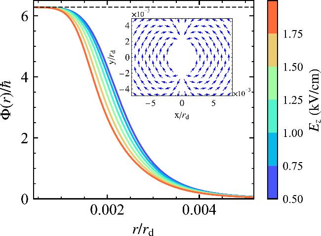
Figure 4. Total magnetic flux Φ(r) across the equator outside a radius r for different static E-field strength Ez. The gray dashed line marks Φ = 2$\pi$. Parameters are Δ = (2$\pi$)10 MHz and Ωr ≡ Ω/Δ = 2. The inset shows a magnetic field distribution in the xz plane for r > rc at Ez = 1.5 kV cm-1. The critical static E-field strength are approximately given by ${E}_{z}^{(1)}\approx 0.81$ kV cm-1 and ${E}_{z}^{(2)}\approx 1.98$ kV cm-1. |
Although this trend holds locally, the static E-field Ez also shifts the shielding radius rc, to which Φc is highly sensitive, and consequently exhibits three distinct regimes as the static E-field Ez is increased. As shown in figure 5, for a weak static E-field with ${E}_{z}\lt {E}_{c}^{(1)}$, Φc decreases with increasing Ez, and vanishes at ${E}_{c}^{(1)}$. For an intermediate static E-field with ${E}_{c}^{(1)}\lt {E}_{z}\lt {E}_{c}^{(2)}$, Φc increases with Ez and saturates to 2$\pi$ as Ez approaches ${E}_{c}^{(2)}$. For sufficiently strong static E-fields with ${E}_{z}\gt {E}_{c}^{(2)}$, rc is no longer well defined, and consequently neither is Φc.
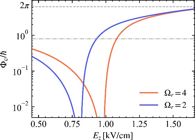


Figure 5. Total magnetic flux across the equator in the regime outside of the shielding core rc as a function of Ez for Ωr = 2 (blue) and Ωr = 4 (orange), respectively, with detuning Δ = (2$\pi$)10 MHz. The dotted-dashed line indicates the maximum value achievable with microwave dressing alone, and gray dashed line labels 2$\pi$. The critical static E-field strength are approximately ${E}_{c}^{(1)}=0.81$ kV cm-1 for Ωr = 2, ${E}_{c}^{(1)}=0.98$ kV cm-1 for Ωr = 4, and ${E}_{c}^{(2)}=1.98$ kV cm-1 for both cases. |
In the absence of a static E-field, the microwave dressing alone yields Φc/ℏ ≲ 0.8. By contrast, tuning the static E-field in the dipolar regime readily enhances Φc/ℏ and allows it to approach 2$\pi$. Moreover, in this regime, reducing Ωr further increases Φc and simultaneously leads to a larger shielding radius rc as indicated in figure 2(d).
4. Conclusion
We investigate the effective potential and the synthetic mutual gauge field of ultracold molecules in a static E-field together with a σ+-polarized microwave. We find that when the static E-field intensity is below the upper critical value ${E}_{c}^{(2)}$, a short-range repulsive core persists and shielding remains effective. As the static E-field is increased across the lower critical value ${E}_{c}^{(1)}$, the long-range interaction crosses over from anti-dipolar to dipolar, with the effective potential becoming fully repulsive at the lower critical point. When the static E-field strength is above ${E}_{c}^{(2)}$, however, the effective potential become purely attractive along the z axis, resulting in the breakdown of 3D shielding. Moreover, the magnetic flux on the equatorial plane outside the shielding radius is highly tunable and can be varied from zero up to values approaching 2$\pi$.