Welcome to visit Communications in Theoretical Physics,
Statistical Physics, Soft Matter and Biophysics

Accurate inference of community structures in networks using variational autoregressive neural networks

  • Shengtong Ma 1, 2, 3 ,
  • Pan Zhang , 1, 2, 3, *
Expand
  • 1School of Fundamental Physics and Mathematical Sciences, Hangzhou Institute for Advanced Study, UCAS, Hangzhou 310024, China
  • 2CAS Key Laboratory for Theoretical Physics, Institute of Theoretical Physics, Chinese Academy of Sciences, Beijing 100190, China
  • 3University of Chinese Academy of Sciences, Beijing 100190, China

*Author to whom any correspondence should be addressed.

Received date: 2026-04-15

  Revised date: 2026-04-29

  Accepted date: 2026-04-30

  Online published: 2026-05-22

Supported by

National Natural Science Foundation of Chinahttp://dx.doi.org/10.13039/501100001809

Copyright

© 2026 Institute of Theoretical Physics CAS, Chinese Physical Society and IOP Publishing. All rights, including for text and data mining, AI training, and similar technologies, are reserved.
This article is available under the terms of the IOP-Standard License.

Abstract

Maximizing modularity is a standard approach for community detection, but it often suffers from a rugged energy landscape and the tendency to overfit random noise. To overcome these limitations, we formulate community detection as a statistical inference problem based on generative models. By modeling the network generation through a degree-corrected stochastic block model, inferring the latent community structure equates to maximizing the model's log-likelihood. Crucially, we show that this likelihood objective is formally equivalent to characterizing the Boltzmann distribution of a spin glass system, where the energy function maps to the negative modularity. To capture this intractable high-dimensional distribution, we propose the variational autoregressive network (VAN) approach to approximate. Unlike traditional belief propagation which relies on tree-like structures, or naive mean field which ignores correlations, our autoregressive framework explicitly captures high-order node dependencies and remains robust in networks with dense local loops. Moreover, in benchmark tests across 12 real-world networks, VAN demonstrates a strong ability to overcome local energy barriers, achieving modularity scores that consistently surpass those of several other baseline algorithms including Louvain, Clauset-Newman-Moore, and LN. Furthermore, by evaluating the marginal entropy of the learned distribution, VAN strictly quantifies microscopic assignment confidence to identify 'topological hesitators' and assess the network's overall structural complexity. Consequently, our method not only recovers statistically significant community structures with competitive modularity but also autonomously determines the effective number of communities and naturally encodes hierarchical network organization.

Cite this article

Shengtong Ma , Pan Zhang . Accurate inference of community structures in networks using variational autoregressive neural networks[J]. Communications in Theoretical Physics, 2026 , 78(8) : 085601 . DOI: 10.1088/1572-9494/ae66ce

1. Introduction

Community detection, or node clustering, is a fundamental problem in modern network science, with wide-ranging applications in social sciences, biology, and computer science [1-5]. It aims to partition the vertices of a graph into groups such that internal connections within groups are denser than external connections. A popular measure for evaluating the quality of such partitions is modularity, which compares the density of edges within communities to that expected in a random null model [6]. Standard approaches typically treat community detection as an optimization problem, seeking a single partition that maximizes modularity [7, 8].
However, maximizing modularity directly presents significant challenges. As highlighted by Zhang and Moore [9, 10], the landscape of modularity is often rugged and 'glassy,' characterized by a large degeneracy of high-modularity partitions that may be poorly correlated with one another. Furthermore, modularity maximization is prone to overfitting; it often identifies illusory 'communities' in sparse random graphs where no true structure exists, finding partitions with modularity scores indistinguishable from those of structured networks [9, 11, 12]. Consequently, a single 'optimal' partition found by greedy or heuristic maximization may merely reflect random noise rather than statistically significant structure [13].
To address these limitations, we adopt a rigorous statistical inference perspective. Assuming that any given network is generated by a sufficiently expressive generative model, community detection fundamentally becomes the inference of the model's parameters-most notably, the underlying node partition. Specifically, we consider the degree-corrected stochastic block model (DCSBM) as the generative framework [3, 9]. Under specific parameter constraints, maximizing the log-likelihood of the DCSBM is mathematically equivalent to maximizing modularity. This equivalence naturally bridges statistical inference with statistical physics, mapping the community detection problem perfectly onto the study of spin glass systems [14, 15]. Instead of seeking a single optimal partition, we focus on the Boltzmann distribution of the system configurations at finite temperature, where the energy function is defined based on the negative modularity. This equivalence grounds our method in rigorous statistical inference: by characterizing the Boltzmann distribution, we are effectively performing Bayesian inference on the generative parameters of the network structure, rather than simply optimizing a quality function.
A key challenge in this probabilistic approach is the intractable calculation of the partition function and the high-dimensional joint distribution. While Markov Chain Monte Carlo methods can sample from the distribution, they suffer from slow mixing times. Message-passing algorithms, such as belief propagation (BP), have been successfully applied to infer the marginals and determine the detectability phase transitions in the SBM [9, 16-18]. However, BP relies on the cavity assumption, which strictly holds only for locally tree-like structures. In real-world networks with short loops and dense local connectivity, the independence assumption of BP breaks down, potentially leading to non-convergence or inaccurate estimations [19]. Conversely, the naive mean field (NMF) approximation simplifies the problem by assuming full independence among variables, but it fails to capture the crucial correlations between node assignments [20].
In this work, we propose a novel approach using variational autoregressive networks (VANs) to approximate the Boltzmann distribution of network partitions [21]. Building on recent advances in deep generative models [22, 23], our method parameterizes the joint probability distribution as a product of conditional probabilities. Unlike NMF, the autoregressive structure explicitly models high-order dependencies and long-range correlations between vertices [24, 25]. By minimizing the variational free energy, VAN effectively searches for the consensus of high-modularity partitions, avoiding the pitfalls of single-point optimization.
Our approach offers several distinct advantages. First, it is robust to the topology of the graph, performing well even in networks with high cyclomatic complexity where BP struggles. Second, our framework allows for the autonomous determination of the number of communities. By setting a sufficiently large upper bound, the entropy term in the free energy naturally suppresses redundant groups. Finally, we demonstrate that the learned variational distribution encodes hierarchical information, enabling the detection of sub-structures without recursive re-optimization [26]. We validate our method on both synthetic benchmarks and real-world networks, showing that it achieves competitive modularity and superior inference accuracy compared to established baselines.

2. Model and methods

2.1. Community partition and spin states
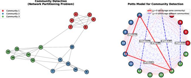
Given a graph constructed with vertices and edges, community detection aims to find a good partition of the vertices (see figure 1 left). This entails determining both the number of groups and the assignment of vertices to the same group. While traditionally viewed as an optimization or clustering problem, it can be formulated as a statistical inference task. If we posit that a generative model possesses sufficient expressive power, any observed graph can be assumed to be generated by this model under specific parameters. Consequently, community detection is fundamentally the inverse problem: inferring these latent parameters from the observed topology, with the group assignment (or node partition) being the most critical parameter to infer. We consider the DCSBM as this underlying generative framework.
Figure 1. (Left) Partition of community detection problem with 3 groups. (Right) Potts model with 3 spins, the spin glass analogy of group assignment partition. Those high lighted edges are examples of how Jij for edge (i, j) effect states (partitions) of both nodes.
We consider the DCSBM as the underlying generative framework. The DCSBM overcomes the limitation of the standard SBM, which typically forces high-degree and low-degree nodes into different groups, by introducing degree parameters $\{k_i\}$ to model the expected degree of each node. Given a partition σ where $\sigma_i \in \{1, \dots, q\}$ denotes the group assignment of node i, the number of edges Aij between nodes i and j follows a Poisson distribution with mean $k_i k_j \omega_{\sigma_i \sigma_j}$, where $\omega$rs is the mixing matrix representing parameters affect connection probabilities between groups r and s.
The inference of the optimal partition corresponds to maximizing the log-likelihood of the observed network structure given the model parameters. For a simple graph, the log-likelihood $L(\boldsymbol{\sigma})$ can be derived as:
$align$
Assuming a simplified structure where $\omega_{rs} = \omega_{\mathrm{in}}$ if r = s and $\omega_{rs} = \omega_{\mathrm{out}}$ if rs, the log-likelihood can be rewritten (up to a constant independent of σ) as:
$align$
By setting specific parameters such that $k_i k_j \frac{\omega_{\mathrm{in}} - \omega_{\mathrm{out}}}{\ln (\omega_{\mathrm{in}}/\omega_{\mathrm{out}})} = \frac{k_i k_j}{2m}$ and identifying the inverse temperature $\beta = \ln(\omega_{\mathrm{in}}/\omega_{\mathrm{out}})$, we find that the log-likelihood is directly proportional to the modularity Q of the partition:
$align$
where $Q(\boldsymbol{\sigma}) = -\frac{1}{2m} \sum_{i \neq j}\left(A_{i j}-\frac{k_i k_j}{2 m}\right) \delta\left(\sigma_i, \sigma_j\right)$. This equivalence implies that the posterior distribution of the partition follows a Boltzmann distribution $P(\boldsymbol{\sigma}) \propto \mathrm{e}^{\beta m Q(\boldsymbol{\sigma})}$. Consequently, the problem of inferring the community structure maps perfectly onto finding the ground state of a spin glass system, specifically a Potts model, with an energy function defined as $E(\boldsymbol{\sigma}) = -m Q(\boldsymbol{\sigma})$.
Following this paradigm, we adopt the Potts model (see figure 1 right) as our foundational framework. The energy function is formally defined as:
$align$
where the coupling strength Jij is derived from the modularity formulation:
$align$
Here, the coupling term $J_{ij} = \frac{1}{2m} (A_{ij} - \frac{k_i k_j}{2m})$ encourages node co-assignment when actual connections exist ($A_{ij} = 1$) and penalizes assignments that contradict the expected connection probability $\frac{k_i k_j}{2m}$ under the configuration null model. Through this derivation, we successfully map the community detection problem of a given graph (figure 1 left) to a fully connected Potts model (figure 1 right), where the ground state corresponds to the partition with maximum modularity.

2.2. Distribution better than single optimum
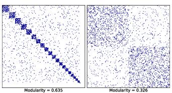
Most traditional community detection methods rely on modularity maximization algorithms, aiming to identify a single optimal partition characterized by high modularity. However, numerous studies have demonstrated that the single optimum derived from modularity maximization often fails to recover the true community structure in networks where ground truth is available. Furthermore, as shown in figure 2, even when distinct communities are genuinely present, the modularity of the true partition is frequently not statistically distinguishable from that of random graphs. Consequently, the single result yielded by modularity maximization is often statistically insignificant.Therefore, rather than seeking a single partition with high modularity, we advocate for identifying a consensus among multiple high-modularity partitions. In statistical physics, for a system consisting of classical particles where interactions depend on their states, the configuration of particle states follows the Boltzmann distribution:
$align$
where $Z = \sum {\mathrm{e}}^{-\beta E(\boldsymbol{\sigma})}$ is the partition function, and $p(\boldsymbol{\sigma})$ represents the joint distribution of the configuration $\boldsymbol{\sigma} = \{1,\dots,q\}^N$, with N denoting the number of particles. Theoretically, if the Boltzmann distribution could be computed exactly, one could determine the probability of each configuration and readily identify those corresponding to low-energy states.
Figure 2. Comparison of modularity maximization on random and structured networks. The adjacency matrices of two networks with N = 1000 nodes and average degree c = 3. Non-zero elements (edges) are shown as dots. (Left) An Erdős-Rényi (ER) random graph sorted by communities found using a greedy modularity maximization algorithm. Despite lacking true community structure, the algorithm 'discovers' illusory communities with a high modularity (Q ≈ 0.635). (Right) A network generated by the stochastic block model (SBM) with true community structure ($c_{\mathrm{out}}/c_{\mathrm{in}} = 0.2$), sorted by its ground truth partition. The modularity of the true partition (Q ≈ 0.326) is lower than that of the random graph's optimized partition, illustrating that maximizing modularity can lead to overfitting on random noise.
In the context of community detection, we map the graph to a spin glass model with the system energy function defined as $E_{\mathrm{partition}}(\{\boldsymbol{\sigma}\})$. Thus, computing the partition function Z becomes the critical step required to obtain the Boltzmann distribution for a given graph. However, the exact computation of Z is #P-hard, necessitating the use of approximation techniques as introduced below.

2.3. Variational autoregressive method

To circumvent the intractability of the partition function, various approximation techniques can be employed, with variational approaches being particularly prominent. The variational method posits a parameterized trial distribution (ansatz), denoted as $q_{\theta}(\boldsymbol{\sigma})$, and seeks to optimize the parameters θ such that $q_{\theta}(\boldsymbol{\sigma})$ approximates the true Boltzmann distribution $p(\boldsymbol{\sigma})$ as closely as possible.
The proximity between the trial and target distributions is quantified using the Kullback-Leibler (KL) divergence, defined as:
$align$
From a statistical mechanics perspective, minimizing the KL divergence is equivalent to minimizing the variational free energy Fq, which is given by:
$align$
Crucially, since the exact free energy of the system, F is constant with respect to the variational parameters θ, optimizing $D_\mathrm{KL}$ is mathematically identical to minimizing Fq. This allows us to optimize the parameters based solely on the energy function $E(\boldsymbol{\sigma})$ without requiring knowledge of the intractable constant F. Furthermore, the non-negativity of the KL divergence implies that $F_q \unicode{x2A7E} F$. Thus, the true free energy F serves as a thermodynamic lower bound, preventing the variational free energy from diverging to negative infinity during optimization.
In this work, we implement this framework using VANs. The VAN approach decomposes the high-dimensional joint probability of the configuration into a product of conditional probabilities using the chain rule:
$align$
By treating the variational parameters θ as weights and biases of the neural network and the variational free energy as part of loss function, VANs enable the effective optimization of θ while explicitly modeling the complex correlations between variables, ultimately yielding a high-fidelity approximation of the Boltzmann distribution.

2.3.1. Masked autoencoder for distribution estimation (MADE).
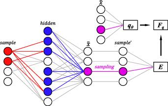
A variety of autoregressive architectures, including RNNs, NADE, and PixelCNN, are applicable to our method. Here, we adopt the MADE [22] due to its implementation efficiency and robust probabilistic modeling capabilities. MADE modifies a standard autoencoder by applying binary masks to the weight matrices, thereby enforcing the autoregressive property where each output dimension depends exclusively on previous dimensions. The specific MLP implementation of MADE used in this work is depicted in figure 3.
Figure 3. Multilayer perceptron (MLP) in 2 layer width with MADE. An initial spin configuration is input as a sample to the network. The colored sites denote the receptive field of a site in sample′, which is sampled from the possibility distribution $\tilde{x}$. We could extend the depth by connecting $\tilde{x}$ with an activation function tanh and the output would be the input to next layer.

2.3.2. Multi-channel sampling.

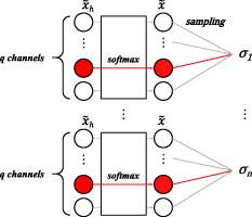
Conceptually analogous to the channel mechanism in convolutional neural networks (CNNs)-where, for instance, three separate channels (R, G, B) encode the intensity values of a pixel-we extend the MADE by introducing a multi-channel architecture. Specifically, we incorporate q channels to model the probability distribution of each vertex belonging to one of the q potential communities, as depicted in figure 4.
Figure 4. Expanded output architecture of MADE. The representation for each node is expanded into q channels to model the probability distribution over q communities. The red highlighted sites illustrate the computational flow for determining the probability of assigning node 1 and node n to a specific group (e.g. the $(q-1)$th group). A softmax layer normalizes the logits across the q channels to produce a valid probability distribution for each node, from which the final discrete state σ is sampled.
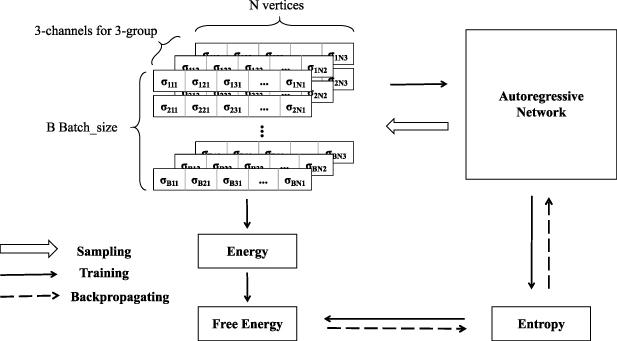
The sampling process is further detailed in figure 5. Each sampling step yields a tensor σ with elements $\sigma_{b,i,k}$, representing the discrete sampled state of node i assigned to group k within batch b. By averaging these binary outcomes over the batch dimension, we derive the estimated marginal probability vector for node i, denoted as $\bar{\boldsymbol{\sigma}}_i = (\bar{\sigma}_{i,1}, \bar{\sigma}_{i,2}, \dots, \bar{\sigma}_{i,q})$, satisfying the condition $\sum_{k = 1}^q \bar{\sigma}_{i,k} = 1$. Consequently, the final group assignment σi for node i is determined by selecting the group with the highest marginal probability:
$\begin{align} \sigma_i = \operatorname*{argmax}_{k \in \left\{1, \dots, q\right\}} \bar{\sigma}_{i,k}.\end{align}$
Figure 5. Multi-channel autoregressive framework and variational inference. We illustrate the process using an example graph with N vertices and 3 groups. The sample size (batch size) is denoted by B. The element $\sigma_{b,i,k} \in \{0,1\}$ represents the sampling outcome for vertex i assigned to group k in batch b. During the training process, sampling is performed based on a categorical distribution.
This multi-channel design enables the model to effectively generate normalized probability distributions over the q groups for every vertex. By leveraging parallel computation across multiple batches, this mechanism not only ensures computational efficiency but also significantly enhances the statistical robustness of the inferred community assignments.

3. Numerical experiments

3.1. Synthetic networks
We evaluate our method on synthetic networks generated by the DCSBM and the standard SBM. In the general formulation of the DCSBM, the number of edges x between node i and node j is drawn from a Poisson distribution:
$\begin{align} P\left(A_{ij} = x\right) = \frac{\lambda_{ij}^x {\mathrm{e}}^{-\lambda_{ij}}}{x!}, \quad \text{with } \lambda_{ij} = k_i k_j \omega_{\sigma_i \sigma_j},\end{align}$
where ki is the degree expectation of node i, $\sigma_i \in \{1, \dots, q\}$ is the group assignment, and $\omega$rs represents the mixing matrix.
For simplicity, we focus on simple graphs which are undirected, contain no multi-edges, and have no self-loops. In this setting, the adjacency matrix entry Aij (for ij) takes values in $\{0, 1\}$. Deriving from equation (11), the probability of observing an edge (i.e. x = 1) is explicitly given by:
$\begin{align} P\left(A_{ij} = 1\right) = \lambda_{ij} {\mathrm{e}}^{-\lambda_{ij}} = k_i k_j \omega_{\sigma_i \sigma_j} {\mathrm{e}}^{-k_i k_j \omega_{\sigma_i \sigma_j}}.\end{align}$
This expression includes the exponential term $\mathrm{e}^{-\lambda_{ij}}$, which ensures proper normalization. However, in the regime of sparse graphs where the connection intensity is low ($\lambda_{ij} \ll 1$), the probability of generating multiple edges in the Poisson process becomes negligible, and the exponential term approaches unity ($\mathrm{e}^{-\lambda_{ij}} \approx1$). Consequently, the edge existence probability can be approximated by the linear form:
$\begin{align} P\left(A_{ij} = 1\right) \approx k_i k_j \omega_{\sigma_i \sigma_j}.\end{align}$
When the degree heterogeneity is removed by setting $k_i = 1$ for all i, the connection probability depends solely on the group memberships, i.e. $P(A_{ij} = 1) \approx \omega_{\sigma_i \sigma_j}$, and the model degenerates to the standard SBM.
To systematically control the detectability of the community structure, we adjust the ratio of intra-community to inter-community connection strengths, defined as $\rho = \omega_{\mathrm{in}} / \omega_{\mathrm{out}}$ (equivalent to $p_{\mathrm{in}}/p_{\mathrm{out}}$ for SBM). For a network with N nodes and q groups of equal size, we fix the average degree c and the ratio ρ to determine the specific values of $\omega_{\mathrm{in}}$ and $\omega_{\mathrm{out}}$.
For the standard SBM, the average degree c is derived by summing the expected connections for a node. Ignoring finite-size corrections (order $1/N$) due to the absence of self-loops, we have:
$\begin{align} c \approx \frac{N}{q} \omega_{\mathrm{in}} + \frac{N\left(q-1\right)}{q} \omega_{\mathrm{out}}.\end{align}$
Substituting $\omega_{\mathrm{out}} = \omega_{\mathrm{in}}/\rho$, we obtain the expression for $\omega_{\mathrm{in}}$ in the SBM:
$\begin{align} \omega_{\mathrm{in}}^{\mathrm{SBM}} = \frac{c \cdot q}{N \left( 1 + \frac{q-1}{\rho} \right)}.\end{align}$
For the DCSBM, the expected degree of a node i is scaled by its propensity ki. Assuming the degree parameters are uncorrelated with group assignments, the empirical average degree of the generated network is scaled by the squared average of the degree parameters, denoted as $\langle k \rangle^2 = (\frac{1}{N}\sum k_i)^2$. The relationship between the target average degree c and the mixing parameter is derived as:
$\begin{align} c_{\mathrm{DCSBM}} \approx \frac{1}{N} \sum_{i \neq j} k_i k_j \omega_{\mathrm{avg}} \approx N \langle k \rangle^2 \omega_{\mathrm{avg}}.\end{align}$
Therefore, to maintain the same sparsity c as the SBM baseline, the affinity parameter $\omega_{\mathrm{in}}$ for DCSBM must be normalized by the second moment of the degree distribution:
$\begin{align} \omega_{\mathrm{in}}^{\mathrm{DCSBM}} \approx \frac{\omega_{\mathrm{in}}^{\mathrm{SBM}}}{\langle k \rangle^2} = \frac{c \cdot q}{N \langle k \rangle^2 \left( 1 + \frac{q-1}{\rho} \right)}.\end{align}$
In our experiments, we sample ki from a Gamma distribution $k_i \sim \Gamma(3c, 1/c)$ to introduce degree heterogeneity, and then apply equation (17) to determine the model parameters, ensuring a fair comparison across different noise levels ρ.
Using the generative models defined above, we conducted extensive experiments to benchmark the inference accuracy and robustness of VAN against baseline methods (BP and NMF).
Inference accuracy and free energy.
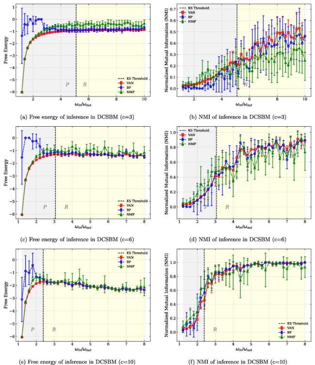
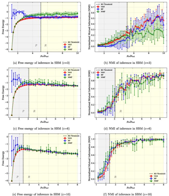
Figures 6 and 7 present the comparative results on SBM and DCSBM networks with N = 100 and c = 3. We vary the signal-to-noise ratio ρ (plotted as $p_{\mathrm{in}}/p_{\mathrm{out}}$ in SBM and $\omega_{\mathrm{in}}/\omega_{\mathrm{out}}$ in DCSBM) to cover the range from the undetectable phase to the clear community structure phase, spanning across the theoretical detectability threshold known as the Kesten-Stigum (KS) bound (see appendix F for the exact derivation). According to equation (3), we apply the same inverse temperature $\beta = \ln\rho$ for all three methods.
Figure 6. Inference on SBM networks. Each data point represents the average result over 10 independent network generated by models under the same parameters. All with N = 100, q = 3. As the community structure becomes more pronounced (increasing $p_{\mathrm{in}}/p_{\mathrm{out}}$), VAN consistently identifies solutions with significantly lower variational free energy and stabler NMI (shorter error bar) compared to BP and naive mean field (NMF).
Figure 7. Inference on DCSBM networks. Each data point represents the average result over 10 independent network generated by models under the same parameters. All with N = 100, q = 3. The expected degrees sampled from $\theta_i \sim \Gamma(3c, 1/c)$. As the community structure becomes more pronounced (increasing $\omega_{\mathrm{in}}/\omega_{\mathrm{out}}$), VAN consistently identifies solutions with significantly lower variational free energy and stabler NMI (shorter error bar) compared to belief propagation (BP) and naive mean field (NMF).
As shown in the Free Energy and NMI plots, the performance of the algorithms varies drastically across the phase transition. Prior to crossing the KS bound (the weak-signal/undetectable phase), the BP algorithm exhibits extreme instability with massive error bars. This occurs because BP fundamentally relies on the cavity assumption; in this dense and noisy regime, it fails to find sufficiently informative tree-like structures, causing the message-passing dynamics to fluctuate wildly or fail to converge. Conversely, well beyond the KS bound where the community structure becomes pronounced, the NMF method paradoxically suffers a degradation in stability and accuracy. This failure stems from NMF's core assumption of variable independence, which critically ignores the increasingly strong topological correlations between nodes as the true communities crystallize.
In sharp contrast, VAN demonstrates exceptional stability and accuracy across both thermodynamic phases. By explicitly capturing high-order node dependencies without relying on fragile tree-like approximations, VAN consistently navigates the rugged phase space to accurately pinpoint the variational distribution with the lowest free energy. This thermodynamic advantage translates directly into superior and stable inference fidelity (remarkably short error bars), particularly in the DCSBM case where degree heterogeneity further confounds standard mean-field methods.
Model selection.
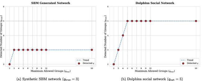
A critical advantage of our autoregressive framework is its ability to automatically determine the effective number of communities ($q^*$) without prior knowledge. Figure 8(a) illustrates this capability on an SBM network generated with a ground truth of $q^* = 3$ groups. Even when the hyperparameter $q_{\mathrm{max}}$ (the maximum allowed number of groups) is increased from 3 up to 20, the number of communities detected by VAN ($q_{\mathrm{VAN}}$) remains stable at 3. Unlike traditional maximum likelihood methods that tend to overfit by utilizing all available parameters, the entropy term in our variational objective naturally penalizes redundant groups, effectively 'pruning' the excess capacity. This result confirms that VAN can perform robust model selection autonomously, a feature that we further validate on real-world networks in the following section.
Figure 8. Autonomous determination of the effective number of communities ($q^\star$) using VAN. The plots illustrate the robustness of our method against the hyperparameter $q_{\mathrm{max}}$. (a) On a synthetic graph generated by SBM with a ground truth of 3 groups, setting (N = 100, c = 3, η = 6.0), the detected number of communities accurately converges to 3 and remains stable even as $q_{\mathrm{max}}$ increases. (b) On the real-world Dolphins social network, the model identifies an optimal structure with 5 groups and avoids overfitting, maintaining this result despite the expansion of the search space ($q_{\mathrm{max}}$). These results demonstrate that VAN can effectively infer the intrinsic community structure without requiring an exact prior on the number of groups.
Unveiling topological hesitators.
Unlike pure optimization heuristics that output a single deterministic hard partition, the VAN framework intrinsically characterizes the entire Boltzmann distribution of the network configurations. This profound capability allows us to move beyond mere macroscopic classification and strictly quantify the microscopic assignment confidence of individual vertices through their marginal entropy.
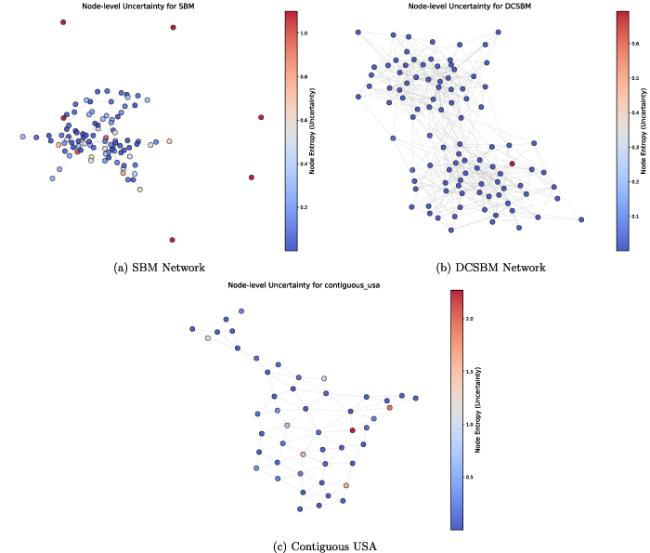
By evaluating the marginal entropy derived from the continuous probabilities of the autoregressive network, we can identify topological hesitators-nodes exhibiting high assignment uncertainty (colored red in figure 9). Physically, these hesitators typically correspond to marginalized isolated vertices or inter-community 'centrists'. For instance, in the synthetic SBM (figure 9(a)), completely isolated nodes lacking connections naturally emerge as obvious hesitators. Additionally, high-entropy outliers arise from the earliest nodes in the autoregressive sequence; lacking prior context, these initial nodes guess randomly to break permutation symmetry, acting as anchors that confer high certainty to subsequently sampled neighbors. Conversely, the DCSBM (figure 9(b)) exhibits such a pronounced community structure that almost all nodes are strictly determined (dark blue, S ≈ 0). The single high-entropy outlier here is merely a mathematical artifact of the autoregressive chain rule, as the unconditionally first sampled node is chosen entirely at random and deterministically guides the rigid alignment of the remaining network.
Figure 9. Quantification of microscopic node-level uncertainty across synthetic and real-world networks. Vertices are colored according to their marginal Shannon entropy, computed directly from the continuous conditional probability distributions inferred by the VAN. (a) A low-noise SBM network (q = 3). (b) A highly structured DCSBM network (q = 2). (c) The empirical Contiguous USA network.
In real-world topologies, such as the Contiguous USA network (figure 9(c)), topological hesitators frequently materialize at the boundaries between distinct groups, reflecting the structural frustration of nodes with ambiguous and competing affiliations. Ultimately, the probabilistic landscape depicted by VAN not only recovers the global community partition but also reveals the microscopic certainty of each constituent. This capability cleanly distinguishes the absolute loyalists secured within a community's core from the true hesitators lingering at phase boundaries, providing significantly deeper insights into network dynamics than standard modularity maximization.
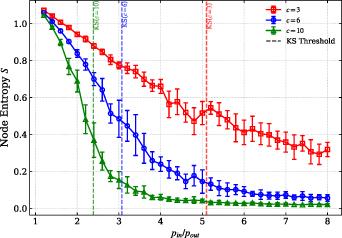
Furthermore, the average nodal entropy serves as a powerful, intrinsic metric for assessing the overall complexity and detectability of the network's community structure. As illustrated in figure 10, in the purely random regime ($p_{{\mathrm{in}}}/p_{{\mathrm{out}}} \to 1$), the lack of structural signal causes the average entropy to saturate near its theoretical maximum ($S \approx \ln 3 \approx 1.1$), reflecting the complete absence of a discernible community structure. As the signal-to-noise ratio increases and the system crosses the KS bound, the average entropy drops precipitously, condensing toward zero deep within the ordered phase. This macroscopic thermodynamic behavior provides a unique statistical physics perspective on the community detection task.
Figure 10. Evolution of average node entropy across the detectability phase transition. The mean marginal entropy, S, evaluated over all nodes in synthetic SBM networks (N = 100, q = 3) is plotted against the signal-to-noise ratio, $p_{\mathrm{in}}/p_{\mathrm{out}}$, for average degrees $c = 3, 6, 10$. Vertical dashed lines indicate the respective theoretical Kesten-Stigum (KS) bounds.
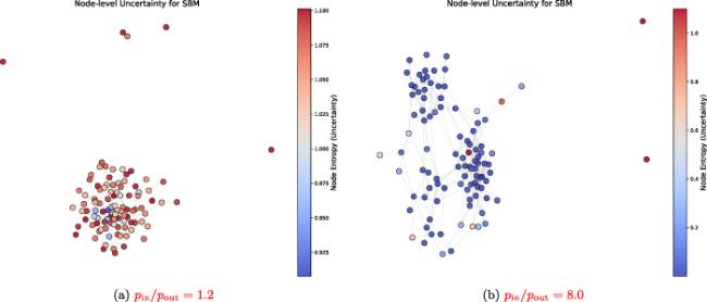
This thermodynamic transition is visually corroborated in figure 11, which contrasts the pervasive uncertainty of an unstructured network against the stark determinism of a highly modular one. At $p_{{\mathrm{in}}}/p_{{\mathrm{out}}} = 1.2$ (figure 11(a)), structural information is overwhelmed by noise, trapping the vast majority of vertices in high-entropy states without genuine allegiance to any global partition. The sporadic presence of isolated low-entropy nodes here is an intrinsic artifact of the autoregressive chain rule: sequential sampling induces strong local correlations, causing a node to deterministically align with its previously sampled neighbors despite the macroscopic randomness. Conversely, at $p_{\mathrm{in}}/p_{\mathrm{out}} = 8.0$ (figure 11(b)), the strong community signal allows the VAN to confidently freeze most nodes into low-entropy states, leaving only isolated vertices and sequence roots as rare hesitators.
Figure 11. Visual comparison of node-level uncertainty at extreme signal-to-noise ratios. Both panels display synthetic SBM networks generated with an identical average degree (c = 6) but differing community strengths: (a) $p_{\mathrm{in}}/p_{\mathrm{out}} = 1.2$, deep within the undetectable phase; (b) $p_{\mathrm{in}}/p_{\mathrm{out}} = 8.0$, well within the detectable phase.

3.2. Real-world networks

To evaluate the practical inference performance of the VAN, we extend our experiments to 12 real-world networks. In the absence of definitive ground-truth partitions for these empirical datasets, we primarily assess the quality of the inferred community structures based on their modularity scores (Q). We compare VAN with the BP, NMF, and heuristic methods including Louvain, Clauset-Newman-Moore (CNM), and LN.
Overall, VAN successfully overcomes the limitations of traditional algorithms on specific topologies and demonstrates a robust capability to find high-modularity configurations. Our detailed analysis is as follows:
Performance in dense local loops.
A defining characteristic of many empirical networks, particularly smaller ones such as 17-Nov and Montreal, is the prevalence of dense short loops. Such topological features strictly violate the tree-like cavity assumption required by BP and the independence assumption of NMF. Consequently, message-passing algorithms frequently fail to converge or yield trivial partitions on these graphs, resulting in modularity scores near or below zero (e.g. $Q_{\mathrm{BP}} = 0$ on 17-Nov and -0.010 on Montreal). In sharp contrast, by leveraging the autoregressive architecture to factorize high-order joint probabilities, VAN circumvents these restrictive assumptions. It maintains stable performance in complex local topologies, achieving modularity scores of 0.284 and 0.335 on the Montreal and Dutch Criticism networks, respectively.
Optimization in the rugged energy landscape.
As shown in table 1, at a precision of three decimal places, VAN consistently matches or slightly exceeds the performance of state-of-the-art heuristic algorithms (such as Louvain and LN) across multiple networks (e.g. Zebras, Karate Club, Polbooks, and Jazz Collab). However, a higher-precision floating-point analysis of the system's energy reveals that VAN is capable of reaching even deeper absolute energy minima (i.e. higher modularity). Specifically:

($\text { ● }$)On the 17-Nov network, VAN achieves $Q = 0.276\,056\,06$, marginally outperforming CNM ($0.276\,056\,01$).

($\text { ● }$)On the Zebras network, VAN yields $Q = 0.276\,803\,86$, slightly higher than LN and Louvain ($0.276\,803\,83$).

($\text { ● }$)On the classic Karate Club network, the score obtained by VAN ($0.444\,9036$) surpasses that of the greedy optimization-based Louvain algorithm ($0.444\,903\,58$).

($\text { ● }$)For the larger Polbooks network, VAN evaluates to $0.527\,20$, improving upon the ∼0.527 00 scores of LN and Louvain.

($\text { ● }$)On the largest and relatively dense Jazz Collab network in our test set (n = 198, m = 2742), where high-order nodal correlations become increasingly complex, VAN reaches a modularity of $0.444\,871\,19$, providing a slight edge over the strong spectral clustering baseline LN ($0.444\,666\,89$).

Table 1. Performance comparison on real-world networks. The columns show the number of nodes (n), edges (m), and the modularity scores (Q) for various algorithms. For VAN, we report results under a unified upper bound of channels $q_{\mathrm{max}}$ (shown in parentheses) without prior knowledge of the true number of communities. The column $q_{\mathrm{VAN}}$ denotes the effective number of communities retained upon convergence. Bold entries indicate the highest modularity achieved on each network (displayed to three decimal places).
Network n m $q_{\mathrm{VAN}}$ ($q_{\mathrm{max}}$) $Q_{\mathrm{VAN}}$ $Q_{\mathrm{BP}}$ $Q_{\mathrm{NMF}}$ $Q_{\mathrm{Louvain}}$ $Q_{\mathrm{CNM}}$ $Q_{\mathrm{LN}}$
17-Nov 22 66 3 (8) 0.276 0.000 0.096 0.275 0.276 -0.024
Zebras 27 111 3 (8) 0.277 0.021 0.256 0.277 0.277 0.277
Karate Club 34 78 4 (8) 0.445 0.065 0.149 0.445 0.411 0.420
Montreal 35 78 4 (8) 0.284 -0.010 -0.116 0.276 0.277 0.282
Dutch Criticism 35 81 3 (8) 0.335 0.015 -0.341 0.326 0.306 0.319
Windsurfers 43 336 2 (8) 0.371 0.369 0.370 0.371 0.365 0.365
Contiguous USA 49 107 4 (8) 0.597 0.469 0.408 0.596 0.582 0.597
Terrorists 911 62 152 6 (8) 0.536 0.225 0.356 0.519 0.500 0.534
Dolphins 62 159 5 (8) 0.529 0.440 0.390 0.519 0.495 0.528
Lesmis 77 254 6 (8) 0.560 0.533 0.361 0.549 0.501 0.560
Polbooks 105 441 5 (8) 0.527 0.518 0.508 0.527 0.502 0.527
Jazz Collab 198 2742 4 (8) 0.445 0.444 0.396 0.436 0.439 0.445
These high-precision numerical results objectively demonstrate that in the deep valleys of the phase space, the combination of a deep generative model and adiabatic annealing effectively prevents the system from being trapped by minor local perturbations. This allows VAN to identify partition configurations that are closer to the theoretical macroscopic extrema than those found by traditional greedy cuts. (Note: on the Lesmis network, VAN achieves $0.560\,008$, which is remarkably close to LN's $0.560\,008\,37$, indicating that both independent paradigms have effectively converged to the same physical pure state).
Robustness of model selection.
Furthermore, a critical feature of VAN is its ability to autonomously determine the effective number of communities ($q^*$) even in real-world networks where the ground truth is unknown. When initialized with a loose upper bound (e.g. $q_{\mathrm{max}} = 8$), VAN does not naively assign nodes to all available groups. Instead, it prunes redundant communities, converging to a smaller, more meaningful set of groups (e.g. finding 3 groups for 17-Nov and 5 for Polbooks). This behavior validates our theoretical argument that the entropy term in the variational free energy naturally regularizes the model, preventing overfitting to the maximum allowed complexity, and is driven by the intrinsic structure of the data rather than the capacity of the ansatz.

3.3. Hierarchical clustering

In complex network analysis, many real-world networks exhibit hierarchical community structures where identified communities may contain further subdivisions into subcommunities. Consequently, the objective of community detection extends beyond identifying a globally optimal partition to revealing these rich internal structures that provide deeper insights into network organization.
Traditional hierarchical community detection approaches typically require recursive application of community detection algorithms on subgraphs corresponding to identified communities. This sequential methodology, while effective, often suffers from computational inefficiency and may not fully capture the intrinsic hierarchical relationships within the network.
Our proposed methodology leverages the variational free energy optimization framework, which yields a variational Boltzmann distribution that encodes comprehensive structural information. This distribution not only identifies the ground state configuration through maximum marginal probabilities-corresponding to the optimal community assignment-but also preserves crucial similarity information through secondary probability maxima.
The hierarchical detection procedure operates as outlined in algorithm 1. First, we apply the VAN to the input graph, obtaining the optimal partition with $q^*$ communities. Subsequently, within each identified community, we perform secondary partitioning based on the secondary maxima of the marginal probabilities. Nodes sharing identical secondary probability states are grouped together, revealing substructures within each primary community. A notable phenomenon observed during this process is the emergence of isolated nodes that form singleton groups during secondary partitioning. We address this by consolidating such isolated nodes into the first subgroup of their respective parent community. This consolidation strategy is theoretically grounded in the interpretation that singleton formations indicate weak associative tendencies. By aggregating these nodes, we preserve the hierarchical integrity of the detected structure.
Algorithm 1. Hierarchical node partitioning.
Require: Node embeddings $\mathbf{X} \in \mathbb{R}^{N \times D}$, Variational distribution $q_\theta(s)$, Initial node groups $\mathcal{G}_0$,Number of hierarchy levels K
Ensure: Hierarchical groups $\mathcal{H} = [\mathcal{G}_1, \mathcal{G}_2, \dots, \mathcal{G}_K]$
1: $\mathcal{H} \gets \emptyset$
2: for level $k \gets 0$ to K - 1 do
3:  $\mathcal{G}_{k+1} \gets \emptyset$
4:  for each group $g \in \mathcal{G}_k$ do
5:   Initialize sub-groups: $\widetilde{g} \gets \{\widetilde{g}^1, \dots, \widetilde{g}^q\}$ as empty sets
6:   for each node $i \in g$ do
7:    Find next best assignment: $t_i = \operatorname{argmax}_{s} q_\theta(s_i)$
8:    Mask current max: $q_\theta(t_i) \gets 0$       $\triangleright$Prepare for next level
9:    Add node i to sub-group $\widetilde{g}^{\mathrm{T}}_{i}$
10:   end for
11:   Remove empty sets from $\widetilde{g}$
12:   $\mathcal{G}_{k+1} \gets \mathcal{G}_{k+1} \cup \widetilde{g}$
13:  end for
14:  $\mathcal{H}.\text{append}(\mathcal{G}_{k+1})$
15: end for
16: return $\mathcal{H}$
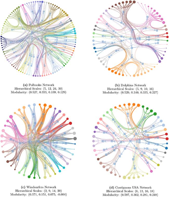
We demonstrate this capability on a diverse set of real-world networks. As visualized in figure 12, our algorithm identifies a hierarchy of scales for each network, starting with the optimal macroscopic partition and recursively subdividing the nodes based on their marginal probabilities. The modularity naturally decreases as granularity increases. Empirically, partitions with $Q \gtrsim 0.3$ denote significant community structure, whereas lower values indicate ambiguous or negligible organization [6]. Consequently, tracking the decay of Q against this threshold provides a quantitative criterion to determine the genuine depth of latent structural hierarchies beyond the initial division.
Figure 12. Hierarchical community structure detection. In the hierarchical diagram, each leaf node represents a community within the network, with its size proportional to the number of nodes it contains. The colors of the leaves and edges indicate the sub-group assignments. The text below each subfigure lists the number of communities (Scales) and the corresponding modularity (Q) at various evolutionary hierarchical levels.
Notably, although the Polbooks network (figure 12(a)) and the Dolphins social network (figure 12(b)) share the same optimal number of primary communities ($q^* = 5$) and similar initial modularities (${\approx}0.53$), their internal organizations differ significantly. The Polbooks network exhibits a deeper progression of scales $(5, 12, 24, 30)$ with a sharp modularity decay, dropping below the 0.3 significance threshold beyond the second level. This suggests a multi-layered but ultimately ambiguous microscopic organization of political alignments. In contrast, the Dolphins network reveals a shallower structural division $(5, 9, 10, 16)$ but maintains meaningful cohesive sub-groups (Q > 0.3) down to the third level.
Furthermore, the hierarchical profiles offer intuitive insights into networks with distinctly different topological origins. The Windsurfers network (figure 12(c)) begins with a valid macroscopic split ($q^* = 2$, Q = 0.371), but any further subdivision immediately falls below the structural significance threshold, indicating a complete lack of robust hierarchical depth. Conversely, the Contiguous USA network (figure 12(d)) starts with a highly modular spatial partition ($q^* = 6$, Q = 0.597) and preserves significant structural integrity (Q = 0.362) at finer scales, reflecting robust geographical sub-clusters before eventually dissolving into local noise.
This comparative analysis highlights that VAN's hierarchical clustering capability provides fine-grained insights into the microscopic structure of complex systems, revealing both the existence and the explicit depth of latent sub-structures that are otherwise completely obscured when evaluating only the global optimal partition.

4. Conclusion

In this work, we have presented a novel probabilistic framework for community detection that rigorously bridges statistical inference, statistical mechanics, and deep learning. Rather than treating community partitioning merely as a heuristic optimization task, we first formulated it as an inference problem based on the DCSBM. We demonstrated that inferring the latent network partition by maximizing the generative model's log-likelihood is mathematically equivalent to finding the ground state of a spin glass system, specifically the Potts model. Driven by this fundamental equivalence, we leveraged VANs to approximate the Boltzmann distribution of the network configurations.
Our theoretical analysis and numerical experiments demonstrate that the VAN approach offers distinct advantages over traditional methods. Unlike the NMF approximation, which assumes variable independence, our autoregressive model explicitly captures high-order dependencies between node assignments. Furthermore, VAN consistently achieves lower variational free energy compared to BP, particularly in empirical networks with dense local loops where the tree-like cavity assumption fatally breaks down.
Our method exhibits robust performance across both synthetic benchmarks and real-world networks, achieving competitive modularity scores alongside classic and widely recognized algorithms such as Louvain, CNM, and spectral methods (LN). It is worth noting that we intentionally did not benchmark against the most aggressive state-of-the-art exact modularity maximizers (such as the Bayan algorithm). As discussed earlier, heuristic modularity maximization algorithms is intrinsically prone to overfitting. Squeezing out marginal numerical advantages in the distant decimal places often reflects the fitting of microscopic random noise rather than the discovery of statistically significant structural features. Thus, comparing our approach against established foundational algorithms provides a far more meaningful validation of its inference accuracy and physical stability.
Crucially, by extracting the marginal entropy from the variational distribution, our framework goes beyond macroscopic partitioning to successfully quantify microscopic assignment confidence. This distinct capability enables the precise identification of 'topological hesitators' lingering at community boundaries and serves as an intrinsic thermodynamic metric for the network's overall detectability across phase transitions.
Beyond robust point estimation, VAN inherently resolves the challenge of model selection. By setting a sufficiently large upper bound for the number of groups, the entropy term in the variational free energy naturally regularizes the model. It autonomously assigns zero probabilities to redundant groups, effectively preventing overfitting. Finally, we demonstrated that the learned variational distribution encodes rich, multi-scale structural information. By evaluating the secondary maxima of the marginal probabilities against a physically motivated significance threshold, we established a natural hierarchical clustering scheme. This approach unveils both the existence and the explicit depth of latent sub-structures without requiring recursive re-optimization.
In summary, VAN provides a powerful, principled, and flexible tool for network analysis. Future work may explore scaling this architecture to massive networks through graph neural network integrations or extending the thermodynamic framework to other combinatorial optimization problems in network science.
A pytorch implementation of our model and algorithms is available at Github: https://github.com/ToothlessMA/infer-commu-van.

Appendix A Autoregressive network

Considering a partition setting q as the upper limit of groups. We have spin configuration $\{\sigma_i^k \}$ equals 1 while node i belongs to group k and 0 otherwise. In autoregressive network, we have a joint probability distribution form

$align$

As a simple example, the joint probability of 4 variables ${\sigma_1^k,\sigma_2^k,\sigma_3^k,\sigma_4^k}$ can be evaluated using Bayes rule as

$\begin{align} & p\left(\sigma_1^k, \sigma_2^k, \sigma_3^k, \sigma_4^k\right) \nonumber\\ = & p\left(\sigma_4^k \mid \sigma_1^k, \sigma_2^k, \sigma_3^k\right) p\left(\sigma_1^k, \sigma_2^k, \sigma_3^k\right) \nonumber\\ = & p\left(\sigma_4^k \mid \sigma_1^k, \sigma_2^k, \sigma_3^k\right) p\left(\sigma_3^k \mid \sigma_1^k, \sigma_2^k\right) p\left(\sigma_1^k, \sigma_2^k\right) \nonumber\\ = & p\left(\sigma_4^k \mid \sigma_1^k, \sigma_2^k, \sigma_3^k\right) p\left(\sigma_3^k \mid \sigma_1^k, \sigma_2^k\right) p\left(\sigma_2^k \mid \sigma_1^k\right) p\left(\sigma_1^k\right). \end{align}$

Meanwhile, with $|k| = 3$ we could have the complete normalization variational distribution with $\sum_k p(\sigma_i^k) = 1$ as follows

$\begin{align} q_\theta\left(\boldsymbol{\sigma}^1\right) &= p\left(\sigma_4^1 \mid \sigma_1^1, \sigma_2^1, \sigma_3^1\right) p\left(\sigma_3^1 \mid \sigma_1^1, \sigma_2^1\right) p\left(\sigma_2^1 \mid \sigma_1^1\right) p\left(\sigma_1^1\right)\nonumber\\ q_\theta\left(\boldsymbol{\sigma}^2\right) &= p\left(\sigma_4^2 \mid \sigma_1^2, \sigma_2^2, \sigma_3^2\right) p\left(\sigma_3^2 \mid \sigma_1^2, \sigma_2^2\right) p\left(\sigma_2^2 \mid \sigma_1^2\right) p\left(\sigma_1^2\right)\nonumber\\ q_\theta\left(\boldsymbol{\sigma}^3\right) &= p\left(\sigma_4^3 \mid \sigma_1^3, \sigma_2^3, \sigma_3^3\right) p\left(\sigma_3^3 \mid \sigma_1^3, \sigma_2^3\right) p\left(\sigma_2^3 \mid \sigma_1^3\right) p\left(\sigma_1^3\right). \end{align}$
To sample a configuration $\boldsymbol{\sigma}^k = \{\sigma_1^k,\sigma_2^k,\sigma_3^k,\sigma_4^k\}$, we first toss a coin to determine $\sigma_1^k$ using marginal probability $p(\sigma_1^k)$, then toss a coin again to determine $\sigma_2^k$ using $p(\sigma_2^k \mid \sigma_1^k)$. The assignment of $\sigma_3^k$ and $\sigma_4^k$ can be determined in turn. After all, we have the final distribution in which
$\begin{align} q_\theta\left(\boldsymbol{\sigma}\right) = \sum_k q_\theta\left(\boldsymbol{\sigma}^k\right) = q_\theta\left(\boldsymbol{\sigma}^1\right)+q_\theta\left(\boldsymbol{\sigma}^2\right)+q_\theta\left(\boldsymbol{\sigma}^3\right).\end{align}$
And after training we take the ground state configuration corresponding $\sigma_i = \text{argmax}_k q_\theta({\sigma_i^k})$.

Building upon this probabilistic framework, the training process involves optimizing the model parameters θ by minimizing the variational free energy. However, a key technical consideration arises: the gradient of the variational free energy $f(\theta)$ cannot be computed directly with respect to the parameters θ due to the discrete nature of the sampling process. To address this challenge, we employ a gradient estimation technique based on the REINFORCE algorithm, which provides an unbiased estimator of the gradient [27, 28]. The mathematical formulation of this gradient estimator is given by:

$align}\begin{aligned}\beta \nabla_\theta F_q & = \nabla_\theta \sum_{\boldsymbol{\sigma}}\left[q_\theta\left(\boldsymbol{\sigma}\right) \cdot\left(\beta E\left(\boldsymbol{\sigma}\right)+\ln q_\theta\left(\boldsymbol{\sigma}\right)\right)\right] \\& = \mathbb{E}_{\boldsymbol{\sigma} \sim q_\theta\left(\boldsymbol{\sigma}\right)}\left[\nabla_\theta \ln q_\theta\left(\boldsymbol{\sigma}\right) \cdot \underbrace{\left(\beta E\left(\boldsymbol{\sigma}\right)+\ln q_\theta\left(\boldsymbol{\sigma}\right)\right)}_{R\left(\boldsymbol{\sigma}\right)}\right]\end{aligned$

In this formulation, each configuration σ sampled from $q_\theta(\boldsymbol{\sigma})$ contributes to the gradient through the term $\nabla_\theta \ln q_\theta(\boldsymbol{\sigma})$, weighted by the reward signal $R(\boldsymbol{\sigma})$. This reward mechanism guides the optimization process: when $R(\boldsymbol{\sigma})$ attains large values, indicating unfavorable configurations with high energy or low probability, the optimizer adjusts the parameters to reduce the likelihood of generating such configurations, thereby systematically lowering the variational free energy.

Appendix B Node-order sensitivity

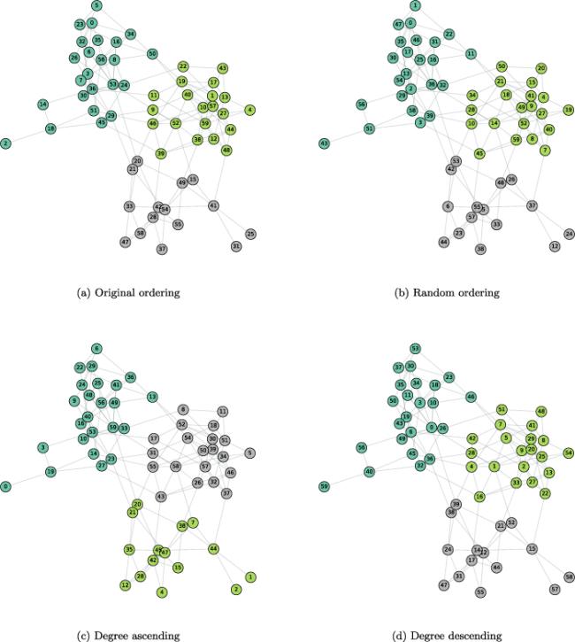
Because the VAN framework generates joint probabilities autoregressively, its inference dynamics inherently depend on the pre-defined node sequence. To systematically evaluate this order sensitivity, we tested four distinct node encodings-original, random, degree ascending, and degree descending-on an identical synthetic SBM network ($N = 60, q = 3, c = 6$) using a fixed random seed. As illustrated in figure 13, the integer labels on the vertices denote the exact generation sequence fed into the autoregressive model. Despite the fundamentally altered local contexts during the sequential sampling process, VAN consistently recovers the exact same optimal partition (indicated by uniform node coloring across all panels) with an identical modularity of $Q = 0.537\,22$. This confirms that our approach is highly robust and invariant to node permutation artifacts.

Figure 13. Robustness of the VAN framework against autoregressive node ordering. The panels display an identical synthetic SBM network evaluated under four distinct autoregressive sequence encodings: (a) the original graph generation ordering, (b) a completely random permutation, (c) sorted by degree in ascending order, and (d) sorted by degree in descending order.

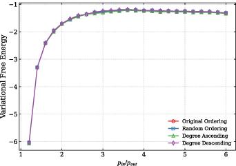
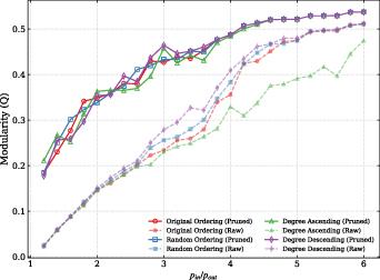
This robustness holds true across the entire thermodynamic phase. As demonstrated in figure 14, the minimized variational free energy shows negligible deviation across all four orderings. The curves nearly perfectly overlap, demonstrating that VAN's capability to locate the deepest energy basins is completely insensitive to the initial node ordering. Furthermore, the pruned modularity (solid lines in figure 15), which tracks the quality of the discovered ground state, remains highly consistent regardless of the input sequence.

Figure 14. Variational free energy across different node orderings. The minimized variational free energy is plotted against $p_{\mathrm{in}}/p_{\mathrm{out}}$ for four distinct input sequences.
Figure 15. Impact of node ordering on modularity optimization. Solid lines represent the pruned modularity (the highest quality partitions found), while dashed lines represent the raw batch-averaged modularity.

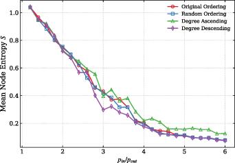
However, the choice of node sequence significantly impacts the network's internal exploration space. Notably, the degree ascending ordering exhibits a massive gap between its raw batch-averaged modularity and its pruned modularity (figure 15). This indicates that starting the autoregressive generation with low-degree (low-information) nodes forces the model to induce a wider, more exhaustive exploration of suboptimal phase spaces before converging. This observation is strongly corroborated by the evolution of mean node entropy in figure 16. While all orderings exhibit a sharp decrease in entropy as the community signal strengthens, the degree ascending sequence visibly maintains a higher average entropy. This quantitatively reflects the increased uncertainty and structural hesitation introduced when the model is forced to condition its earliest sampling decisions on sparsely connected nodes. In conclusion, while node reordering alters the intermediate sampling entropy and exploration volume, VAN's primary macroscopic optimization targets-free energy and optimal partition modularity-are highly robust to the input sequence. Therefore, VAN can operate effectively on complex networks without requiring specialized heuristic pre-ordering.

Figure 16. Evolution of mean node entropy under different autoregressive sequences. The mean marginal Shannon entropy is plotted against $p_{\mathrm{in}}/p_{\mathrm{out}}$ for the four evaluated orderings.

Appendix C Annealing

In spin glass systems, the rugged energy landscape is characterized by a multitude of local minima [29, 30]. Consequently, the inverse temperature β is critical for finding the true ground state. Rather than optimizing at a fixed β, we employ an adiabatic annealing schedule [31] during the autoregressive network training to navigate this glassy landscape and locate the global optimum.

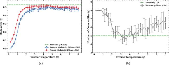
The necessity of this annealing process is demonstrated in figure 17, where we evaluate the VAN approach on the Dolphins social network across various fixed inverse temperatures. Because VAN maintains a vast exploration space, we monitor two metrics to characterize the macroscopic state: Average modularity (the mean over all sampled batches) and Pruned modularity (the mean of the top 10% batches). This pruning filters out thermal noise to isolate the high-quality ground state candidates discovered during exploration.

Figure 17. VAN performance at fixed temperatures vs annealing on the Dolphins social network. Data points represent the mean and standard deviation over 10 independent runs. (a) Average modularity (all batches) and pruned modularity (top 10% batches) as a function of fixed β. (b) The effective number of communities q detected at fixed β. In both panels, the horizontal dashed green lines indicate the stable, optimal results (Q ≈ 0.529, q = 5) achieved through continuous annealing.

The numerical results reveal three distinct thermodynamic regimes, characterized by the modularity, the inferred community count (q), and their statistical fluctuations (error bars):

($\text { ● }$)High-temperature regime ($\beta \lesssim 2$): Entropy dominates, keeping the system in a disordered, paramagnetic-like phase. Modularity is near zero (figure 17(a)), and the model fails to prune redundant groups ($q \approx q_{\mathrm{max}} = 8$, figure 17(b). The small error bars indicate uniform convergence to this highly degenerate state.

($\text { ● }$)Intermediate-temperature regime ($3 \lesssim \beta \lesssim 5$): The system captures the true macroscopic structure. Modularity reaches its peak, and the effective number of communities correctly condenses to $q^\star = 5$.

($\text { ● }$)Low-temperature regime ($\beta \gtrsim 5$): Energy abruptly dominates. A sudden quench to high β prematurely freezes the network into suboptimal local minima. This is evidenced by drastically widened error bars-indicating massive sample-to-sample fluctuations from different random initializations-and a growing divergence between average and pruned modularities, reflecting the fragmented probability distribution typical of spin glasses.

Finding an optimal β window manually for every empirical graph is impractical. By implementing a slow annealing schedule (e.g. linear or logarithmic increment of β), the network smoothly tracks the equilibrium Boltzmann distribution as it cools. As indicated by the dashed green lines in figure 17, the annealed VAN stably converges to the optimal modularity (Q ≈ 0.529) and precise community count (q = 5), effectively bypassing the glassy traps of fixed-β optimization.

Appendix D Naive mean field (NMF) self-consistent equations

This appendix presents the complete derivation of the NMF self-consistent equations for community detection. The mean field free energy is defined as:

$align$
where β is the inverse temperature, $P_{\mathrm{MF}}(\boldsymbol{\sigma})$ is the mean field probability distribution, and $E(\boldsymbol{\sigma})$ is the energy function derived from the modularity Hamiltonian:
$align$

Under the mean field assumption of factorized probability $P_{\mathrm{MF}}(\boldsymbol{\sigma}) = \prod_i P_i(\sigma_i)$, the energy and entropy terms simplify to:

$\begin{align} \begin{aligned} U_{\mathrm{MF}} & = -\frac{1}{2} \sum_q \sum_{i \neq j} P_i\left(q\right) \left(A_{ij} - \frac{k_i k_j}{2m}\right) P_j\left(q\right), \\ S_{\mathrm{MF}} & = -\sum_i \sum_q P_i\left(q\right) \ln P_i\left(q\right). \end{aligned}\end{align}$

The probability distribution is parameterized using auxiliary fields $h_i(q)$:

$align$

Minimizing the free energy with respect to $h_i(q)$ yields the self-consistent equations. The derivatives are computed as:

$\begin{align} \begin{aligned} \frac{\partial U_{\mathrm{MF}}}{\partial h_i\left(q\right)} & = -\frac{\partial P_i\left(q\right)}{\partial h_i\left(q\right)} \sum_{j \neq i} \left(A_{ij} - \frac{k_i k_j}{2m}\right) P_j\left(q\right), \\ \frac{\partial S_{\mathrm{MF}}}{\partial h_i\left(q\right)} & = -\frac{\partial P_i\left(q\right)}{\partial h_i\left(q\right)} \left( \ln P_i\left(q\right) + 1 \right). \end{aligned}\end{align}$

Setting $\frac{\partial F_{\mathrm{MF}}}{\partial h_i(q)} = 0$ and using $\frac{\partial P_i(q)}{\partial h_i(q)} = P_i(q)(1 - P_i(q))$, we obtain:

$align$

Since $h_i(q) = \ln P_i(q) + \text{constant}$ and the constant is absorbed by normalization, the final self-consistent equations are:

$align$

These equations form the basis for the iterative NMF algorithm used in this work.

Appendix E Bethe free energy

The calculation of the free energy serves as a fundamental metric to evaluate how closely the inferred distribution approximates the true Boltzmann distribution of the system. In the thermodynamic framework, the belief propagation (BP) algorithm aims to minimize the variational free energy. Theoretically, the fixed points of BP correspond to the stationary points of the Bethe free energy approximation [12]. A lower free energy indicates a configuration that captures the statistical weight of the true posterior distribution more accurately.

Once the BP messages $\psi_{t}^{i \to k}$ (representing the marginal probability that node i belongs to group t in the absence of neighbor k) have converged, the Bethe free energy density $f_{\mathrm{Bethe}}$ is computed as:

$align$
where n is the number of nodes, m is the number of edges, and $\theta_t = \sum_{j} d_j \psi_{t}^{j}$ is the auxiliary external field representing the mean-field interaction for group t. The terms Zij and Zi serve as local partition functions (normalization constants).

The pairwise normalization term Zij accounts for the interaction between connected nodes i and j:

$align$
where δrs is the Kronecker delta, encouraging nodes in the same community to connect.

The site normalization term Zi incorporates both the external mean field and the incoming messages from the neighborhood $\partial i$:

$align$

It is crucial to observe that the calculation of Zi in equation (E3) relies on the product operation $\prod_{j \in \partial i}$. This mathematical formulation implicitly assumes that the incoming messages from neighbors are statistically independent. This assumption holds strictly only for trees or locally tree-like structures.

However, in networks with short loops or dense cycle structures, this independence assumption is violated. The correlations between neighbors induce a 'self-resonance' effect, where a node's belief feeds back to itself through the loops. Consequently, the factorized form in equation (E3) overestimates the independence of neighbors, leading to an inaccurate estimation of the partition function. Since $f_{\mathrm{Bethe}}$ is directly derived from terms like $\ln Z_i$, the presence of loops causes the calculated free energy to deviate from the true Gibbs free energy. This explains why the BP approximation may degrade in precision for graphs with complex, loopy topologies compared to methods that can capture higher-order correlations.

Finally, to detect community structure, we compare the minimized $f_{\mathrm{Bethe}}$ with the free energy of the trivial factorized state (paramagnetic phase), denoted as $f_{\mathrm{fact}}$. A retrieval phase is identified only when $f_{\mathrm{Bethe}} \lt f_{\mathrm{fact}}$, signifying a statistically significant partition.

Appendix F Kesten-Stigum (KS) bound

The KS bound defines the fundamental theoretical limit for community detectability. Below this threshold, the community signal decays faster than it propagates along the network, rendering the true partition fundamentally indistinguishable from random noise.

For a symmetric stochastic block model (SBM) with N nodes, q groups of equal size, and an average degree c, the expected internal and external connections for a node are $c_{\mathrm{in}}$ and $c_{\mathrm{out}}$, respectively. The overall average degree is constrained by $c = \frac{1}{q} c_{\mathrm{in}} + \frac{q-1}{q} c_{\mathrm{out}}$. The detectability condition, derived from the eigenvalues of the transition matrix on a locally tree-like structure, is strictly given by:

$\begin{align} \left(c_{\mathrm{in}} - c_{\mathrm{out}}\right)^2 \gt q^2 c.\end{align}$

In our numerical experiments, we control the detectability phase by tuning the signal-to-noise ratio, defined as $\rho = p_{\mathrm{in}}/p_{\mathrm{out}} = c_{\mathrm{in}}/c_{\mathrm{out}}$. To establish the exact phase boundary used in our figures, we substitute $c_{\mathrm{in}} = \rho c_{\mathrm{out}}$ into the average degree constraint, yielding $c_{\mathrm{out}} = \frac{q c}{\rho + q - 1}$ and $c_{\mathrm{in}} = \frac{\rho q c}{\rho + q - 1}$.

Substituting these into the fundamental KS condition and solving for ρ yields the explicit critical threshold:

$\begin{align} \rho_{\mathrm{KS}} = \frac{\sqrt{c} + q - 1}{\sqrt{c} - 1}.\end{align}$

This precise equation defines the vertical phase boundary separating the undetectable and detectable phases in our SBM results. It is important to note that for the DCSBM, the introduction of heterogeneous node degree parameters $\{\theta_i\}$ intrinsically alters the local topology. Consequently, while $\rho_{\mathrm{KS}}$ precisely locates the phase transition for the standard SBM, it serves as a robust but approximate analytical boundary for the detectability transition in the DCSBM.

Post-Publication Change (made 03 June 2026). Changes were made to correct the formatting.

We gratefully acknowledge Cheng Ye and Lin Zhou for their valuable discussions and programming suggestions. This work was funded by the Research Funds of the Hangzhou Institute for Advanced Study, University of Chinese Academy of Sciences (UCAS), and supported by the National Natural Science Foundation of China (Grant Nos. 12325501, 12047503, 12247104, 12104056, and 92365206).

1
PorterM A, OnnelaJ-P, MuchaP J2009Communities in networksNotices AMS56 1082

2
FortunatoS2010Community detection in graphsPhys. Rep.486 75

DOI

3
NewmanM E2010Networks: An Introduction Oxford University Press

4
RosvallM, BergstromC T2008Maps of random walks on complex networks reveal community structureProc. Natl Acad. Sci.105 1118

DOI

5
LiS-H, DongC-X, ZhangL, WangL2020Neural canonical transformation with symplectic flowsPhys. Rev. X10 021020

DOI

6
NewmanM E, GirvanM2004Finding and evaluating community structure in networksPhys. Rev. E69 026113

DOI

7
ClausetA, NewmanM E, MooreC2004Finding community structure in very large networksPhys. Rev. E70 066111

DOI

8
BlondelV D, GuillaumeJ-L, LambiotteR, LefebvreE2008Fast unfolding of communities in large networksJ. Stat. Mech.2008 10008

DOI

9
ZhangP, MooreC2014Scalable detection of statistically significant communities and hierarchies, using message passing for modularityProc. Natl Acad. Sci.111 18144

DOI

10
ZhangP, MooreC2016Community detection in sparse networks via grothendieck's inequalityMath. Program.157 181

DOI

11
GoodB H, De MontjoyeY-A, ClausetA2010Performance of modularity maximization in practical contextsPhys. Rev. E81 046106

DOI

12
DecelleA, KrzakalaF, MooreC, ZdeborováL2011Inference and phase transitions in the detection of modules in sparse networksPhys. Rev. Lett.107 065701

DOI

13
ZdeborováL, KrzakalaF2016Statistical physics of inference: thresholds and algorithmsAdv. Phys.65 453

DOI

14
ReichardtJ, BornholdtS2006Statistical mechanics of community detectionPhys. Rev. E74 016110

DOI

15
LucasA2014Ising formulations of many NP problemsFront. Phys.2 5

DOI

16
DecelleA, KrzakalaF, MooreC, ZdeborováL2011Asymptotic analysis of the stochastic block model for modular networks and its algorithmic applicationsPhys. Rev. E84 066106

DOI

17
Von LuxburgU2007A tutorial on spectral clusteringStat. Comput.17 395

DOI

18
KarrerB, NewmanM E2011Stochastic blockmodels and community structure in networksPhys. Rev. E83 016107

DOI

19
WainwrightM J, JordanM I2008Graphical Models, Exponential Families and Variational Inference Now Publishers Inc

20
JordanM I, GhahramaniZ, JaakkolaT S, SaulL K1999An introduction to variational methods for graphical modelsLearning in Graphical Models MIT Press pp 183233

21
WuD, WangL, ZhangP2019Solving statistical mechanics using variational autoregressive networksPhys. Rev. Lett.122 080602

DOI

22
GermainM, GregorK, MurrayI, LarochelleH2015MADE: masked autoencoder for distribution estimationInt. Conf. on Machine Learning PMLR pp 8819

23
NicoliM, PanQ, ZhangP2020Asymptotically optimal variational inference for network reconstructionPhys. Rev. E102 062311

DOI

24
LiuJ-G, LiangL, WangL2021Variational autoregressive networks for solving statistical mechanicsPhys. Rev. E103 033307

DOI

25
PanF, ZhouP, LiS-J, ZhangP2021Contracting tensor networks with graph partitioningPhys. Rev. B103 125137

DOI

26
PeixotoT P2014Hierarchical block structures and high-resolution model selection in large networksPhys. Rev. X4 011047

DOI

27
ZhangP, WangJ, LiH-J2012Comparative study of algorithms for the maximum clique problemPhys. Rev. E85 066708

DOI

28
WangLet al2020Solving quantum statistical mechanics with variational autoregressive networks and quantum circuitsMach. Learn.: Sci. Technol.2 025026

DOI

29
MézardM, ParisiG, VirasoroM A1987Spin Glass Theory and Beyond World Scientific

30
SherringtonD, KirkpatrickS1975Solvable model of a spin-glassPhys. Rev. Lett.35 1792

DOI

31
KirkpatrickS, GelattC D, VecchiM P1983Optimization by simulated annealingScience220 671

DOI

Outlines

/