

1. Introduction
Over the past decades, a wide array of artificial neural network (ANN) models with diverse architectures and characteristics has been widely applied across numerous fields. For instance, feedforward neural networks (FNNs) excel at processing static, structured tabular data and tackling simple classification and regression tasks [1, 2]. In contrast, convolutional neural networks (CNNs) are particularly adept at handling grid-like data such as images and videos [3], while recurrent neural networks (RNNs) show superior performance with sequential data like time series, text, and speech. Among them, reservoir computing (RC) [4, 5], a type of RNN, has attracted notable interest driven by its simple architecture and training efficiency. In contrast to other deep learning models, RC comprises only a single hidden layer, known as the 'reservoir', which can be conceptualized as a complex network of numerous nonlinear oscillators. With the exception of the output layer, whose weights are determined during training based on input data, all other components, such as the input layer and reservoir layer, remain fixed after initial construction. It currently demonstrates superior performance in fields such as speech recognition, robotic control, and time-series prediction [6, 7]. Particularly in forecasting chaotic systems, it can not only accurately predict state evolution beyond six Lyapunov times but also faithfully reconstruct their long-term statistical properties [8-10]. Furthermore, it has proven capable of accurately predicting high-dimensional spatiotemporal systems [11-13], atmospheric systems [14], and critical transition in complex systems [15-17].
Despite demonstrating remarkable performance in a wide range of applications, the underlying mechanisms of RC remain elusive [18-25], representing a fundamental problem pervasive across machine learning. Achieving optimal performance necessitates careful hyperparameter tuning, as some parameters are robust over a broad range while others are highly sensitive. Consequently, the design process often depends on both practical experience and a measure of luck. These uncertainties make investigating the mechanisms of RC critically important. Of course, this indeed faces many difficulties. The predictive performance of RC is not only related to its own structural characteristics but also depends on the dynamics of the target system. Therefore, its mechanism is difficult to explain clearly with a single theory. A widely held view is that the learning of a target system's dynamics by an RC necessitates prior generalized synchronization between them [9, 20]. Empirical studies further indicate that the computational power of RC is maximized at the edge of chaos [21]. Moreover, in tasks involving the memorization of multiple chaotic attractors, the nodes in reservoir network self-organize into separate functional networks [26, 27] that correspond to each individual attractor [28, 29]. In [25], the authors proposed a reconstructed RC framework based on the phase oscillator model. Their results demonstrate that a well-trained model exhibits a power-law distribution in the size of its internal synchronous clusters, a hallmark of criticality. However, the model's capability to achieve generalized synchronization with the target system remains a subject of debate. Furthermore, it underperforms conventional RC in both hyperparameter tuning and predictive accuracy.
In neuroscience, substantial evidence now confirms that criticality serves as the dynamical foundation for many brain functions [30-32]. This is because the brain at criticality achieves an optimal performance in terms of information processing, dynamic range, and energy efficiency [33-36]. When subjected to minor perturbations such as fatigue, pharmacological stimuli, or injury, the brain may deviate from its critical state. However, it can self-correct through various homeostatic mechanisms, including regulation by inhibitory neurons and neuromodulators [37, 38]. This phenomenon is a manifestation of self-organized criticality. Substantial deviations from criticality are implicated in severe neurological conditions: epilepsy is characterized by a super-critical state, while schizophrenia and autism exhibit sub-critical dynamics. Consequently, re-establishing criticality has emerged as a promising strategic goal for future neurological therapies. This leads to a fundamental question: what universal statistical signature is shared by the hypothetical neurons within brain-inspired ANNs that underlies their high predictive efficiency? The discovery of such a signature would provide a principled guideline for the design of more efficient machine models.
Using the traditional RC model as an example, we find that a successfully trained reservoir, defined by its ability to not only predict short-term chaotic evolution but also reconstruct long-term statistics like the strange attractor, exhibits the distinct power-law distribution in the sizes of self-organized synchronous clusters. Furthermore, the scaling of the power-law distribution differs markedly when the RC learns distinct chaotic attractors like the Rössler and Lorenz systems. This indicates that high-performance RC may exhibit critical-like characteristics, wherein learning different tasks leaves a unique signature in the form of a distinct scaling exponent. Then, does RC exhibit the same characteristics when performing more complex tasks? Following [28, 29], we design a multifunctional RC capable of simultaneously memorizing multiple chaotic attractors. A parameter control channel is incorporated into the traditional RC framework. Within this channel, different parameters are assigned to different attractors, enabling the precise retrieval of a target attractor from memory based on specific control inputs. This method, known as parameter-aware RC, has been successfully applied to predict the critical transition of system collapses [16], to identify the critical coupling for synchronization in coupled oscillators [17] and to reconstruct the whole bifurcation process of a chaotic system [39, 40]. We found that the multifunctional RC autonomously reconfigures its cluster size distribution as it retrieves different attractors from memory, resulting in a configuration that is virtually identical to the distribution generated by a traditional RC trained solely on the corresponding attractor.
The rest of the paper is organized as follows. The traditional and multifunctional RC will be articulated in section 2 . The statistical properties from a traditional RC learning the chaotic system will be demonstrated in section 3 . We then report in section 4 the statistical characteristics of the multifunctional RC when simultaneously memorizing multiple chaotic attractors. Finally, section 5 provides the discussion and conclusions.
2. Model
2.1. The traditional RC
The traditional RC, as shown in the lower row of figure 1(a), consists of three modules: the input layer (input to reservoir), the hidden layer (reservoir), and the output layer (reservoir to output). The input layer is defined by the weight matrix $\boldsymbol{W}_{\boldsymbol{\mathrm{in}}}\in\mathbb{R}^{D_\mathrm{r}\times{D_{\mathrm{in}}}}$, which maps the low-dimensional input vector $\boldsymbol{u}(t)\in\mathbb{R}^{D_\mathrm{in}}$ into the high-dimensional reservoir space. Here, $D_\mathrm{in}$ and $D_\mathrm{r}$ denote the dimensions of the input signal and the reservoir, respectively. The reservoir topology is characterized by a sparse random Erdös-Rényi matrix $\boldsymbol{A}\in\mathbb{R}^{D_\mathrm{r}\times{D_\mathrm{r}}}$ with connection density d, whose non-zero entries are populated with random values uniformly distributed in the interval [-1, 1]. The matrix A is rescaled by the spectral radius such that its largest eigenvalue becomes $\mathrm{\lambda}$. The values of $\boldsymbol{W}_{\textbf{in}}$ are randomly selected from a uniform distribution over the interval $[-\sigma, \sigma]$. Once the input vector enters the reservoir, the internal states $\boldsymbol{r}(t)\in\mathbb{R}^{D_\mathrm{r}}$, which can be initialized with random values, are updated as
$equation$
Here, $\Delta{t}$ defines the time step for updating the reservoir, $\alpha\in(0,1]$ is the leaking rate. The machine's output vector, $\boldsymbol{v}(t)\in\mathbb{R}^{D_\mathrm{out}}$, is obtained by coupling the reservoir state through the output matrix $\boldsymbol{W}_{\textbf{out}}\in\mathbb{R}^{D_\mathrm{out}\times{D_\mathrm{r}}}$, which can be described by $equation$
the new state $\boldsymbol{\tilde{r}}\in\mathbb{R}^{D_\mathrm{r}}$ is defined based on the original reservoir state r, that is, $\tilde{r}_{i} = r_{i}$ for the odd nodes and $\tilde{r}_{i} = r^{2}_{i}$ for the even nodes [11].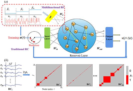
Figure 1. The schematic diagram of a multifunctional RC. (a) The traditional RC architecture comprises an input layer, a reservoir layer, and an output layer, with a reservoir network size $D_\mathrm{r}$ and node states denoted as ri. During training, the RC operates in open-loop mode, whereas in prediction, it switches to closed-loop mode via a bidirectional switch. Multifunctional RC adds a label channel βi compared to traditional RC. It is a step function where different labels are used to mark different attractors. The label is fed into the machine via the $\boldsymbol{W}_{\boldsymbol{b}}$ matrix, while the corresponding ui is fed into the machine via $\boldsymbol{W}_{\textbf{in}}$. During the prediction phase, unlike traditional RC, in addition to replacing the input u with the output v, the βi is continuously fed into the machine. By switching to different labels, different attractors can be reconstructed. (b) Schematic diagram of RC synchronization clusters. Following the method outlined in the main text, M RCs are constructed. Within each RC, synchronization clusters are determined based on the correlation among the time series of all oscillators. Oscillator pairs whose correlation exceeds the preset threshold $p_\mathrm{c}$ are grouped into the same cluster. After reordering all oscillators, the clusters in RCi are represented by the red regions in the figure. |
The training objective of RC is to find an optimal $\boldsymbol{W}_{\textbf{out}}$ that minimizes the error between the L output values and the corresponding input values, such that, $\boldsymbol{v}(t+\Delta{t})\approx{\boldsymbol{u}(t+\Delta{t})}$. Here, L is the length of the training series, and $t = (\tau+1)\Delta{t}\cdot\cdot\cdot(\tau+L)\Delta{t}$, with $T_{0} = \tau\Delta{t}$ ($\Delta{t} = 0.05$) the transient period (to remove the impact of the initial conditions of the reservoir). The total length of the sequence to be observed from the true attractor is denoted by $T = \tau+L$. In the subsequent investigations, we set τ = 100, which is sufficient to eliminate the initial memory of RC. $\boldsymbol{W}_{\textbf{out}}$ can be obtained using a regularized linear regression method, which gives [8, 9]
$equation$
Here, the kth column of the matrix V is the state vector $\boldsymbol{\tilde{r}}[(\tau+k)\Delta{t}]$, $\boldsymbol{U}\in\mathbb{R}^{D_\mathrm{out}\times{L}}$ is also a matrix the kth column of which is $\boldsymbol{u}[(\tau+k)\Delta{t}]$, ξ is the ridge regression parameter for avoiding overfitting, and $\mathbb{I}$ is the identity matrix. As demonstrated above, the hyperparameters of RC include the training sequence length T, the reservoir size ($D_\mathrm{r}$), the connecting density of the reservoir network (d), the range of the input matrix (σ), the leaking rate (a), the spectral radius ($\lambda$) and the regression coefficient (ξ). Upon completion of training, the output matrix ($\boldsymbol{W}_{\textbf{out}}$) retains a static configuration, and the system proceeds to the prediction phase. In this phase, the RC shifts from the open-loop to the closed-loop, where the input vector $\boldsymbol{u}(t)$ is directly replaced by the output vector $\boldsymbol{v}(t)$. Following the common practice in chaotic system prediction, we set $D_\mathrm{out} = D_\mathrm{in}$ [8, 9].2.2. The multifunctional RC
In addition to single-task learning, we design a multifunctional RC, as shown in the upper row of figure 1(a), based on [29] that can simultaneously memorize multiple chaotic attractors. Its state $\boldsymbol{r}(t)$ is updated as 1 ) is the incorporation of a parameter (label) channel $\beta{\boldsymbol{W}_{\boldsymbol{b}}}$ in the multifunctional RC, where $ \beta = \{\beta_{\textit{i}}, \textit{i} = 1,\ldots,m\}$ labels m distinct chaotic attractors to be memorized, and the elements of $\boldsymbol{W}_{\boldsymbol{b}}$ still take values from [$-\sigma,\sigma$]. Furthermore, the training data is substantially different, being composed of two distinct time series, namely the input vector $\boldsymbol{u}(t)$ (formed by states from different attractors) and its corresponding label $\beta(t)$. More specifically, the input vector $\boldsymbol{u}(t)$ with a length of $\hat{T}$ comprises m concatenated time-series segments ($\boldsymbol{u}_{i}(t)$) of equal length Ti (i.e. $ \hat{T} = mT_{i}, T_{i} = \tau+L, i = 1,\ldots,m$), each derived from a distinct attractor to be memorized. The $\mathbf{\beta}_{i}(t)$ is constant and unique for any given attractor but differs across attractors, thereby forming a step function $\mathbf{\beta}(t)$, as shown in figure 1(a). The training procedure remains the same as before, meaning that $\boldsymbol{W}_{\textbf{out}}$ is still given by equation (3 ). However, the vector $\boldsymbol{U}\in\mathbb{R}^{D_\mathrm{out}\times{mL}}$ is now constructed from m input vectors $\boldsymbol{u}_{i}(t)$.
$align$
The primary difference from equation (Differing from prior prediction tasks, the multifunctional RC must reconstruct the specific attractor during prediction phase using only the external cue, the label β. Here, precise prediction of the system's evolution is not required. Alternatively, it can be understood that the RC, having learned multiple attractors during training, must now recall the specific one associated with each distinct cue. This method of memory addressing is termed location-addressable memory in neuroscience [41, 42]. In the following, we provide a detailed description of the memory retrieval process. We begin by arbitrarily selecting a specific label value $\beta\in\{\beta_{i}\}$ and continuously feeding it into the machine. The RC, initialized with random values, can then be treated as an autonomous dynamical system, where the output $\boldsymbol{v}(t)$ at each step is fed back as the next input $\boldsymbol{u}(t)$. From the resulting output $\boldsymbol{v}(t)$, the corresponding attractor can be reconstructed. If the RC successfully reconstructs the attractors associated with different label values βi, we conclude that both the training and retrieval processes have been successful. To quantify whether the RC successfully reconstructs the attractor, we introduce a deviation value [43]: $D = \sum_{i = 1}^{m_{x}}\sum_{j = 1}^{m_{y}}\sqrt{(f_{i,j}-\hat{f}_{i,j})^{2}}$. As defined, we discretize the phase space into a large number of fine cells. Each cell is indexed by (i, j), with $i(j) = 1,\ldots, m_{x}(m_{y})$, where mx = my = 100 are the total numbers of cells along the x and y directions, respectively. The frequencies at which the true trajectory and the predicted trajectory (both of length $\tilde{T}$) visit cell (i, j) are denoted by $f_{i,j}$ and $\hat{f}_{i,j}$, respectively. Theoretically, a smaller deviation value D corresponds to a more accurate attractor reconstruction by the RC. It should be noted that measure D does not represent the actual deviation distance between the predicted trajectory and the real trajectory. In practice, however, D is difficult to approach zero due to the finite length of predicted trajectories and the sensitivity of chaotic systems to initial conditions. To establish a suitable threshold for D, we numerically simulate the chaotic system from two distinct initial conditions. After evolving the system for a sufficient duration (specifically, it refers to $\tilde{T}$ data points), we compute the D0 between the two resulting attractors. This value serves as a benchmark for assessing the RC's reconstruction performance. If the D between the reconstructed and true attractors is close to the D0, i.e. $|D_{0}-D| \lt {D_\mathrm{c}} = 0.1$, the retrieval is deemed successful. $D_\mathrm{c}$ is a tolerance threshold chosen empirically. It is also noteworthy that, as shown in [29], when different labels βi are applied, random initialization of the RC may lead to unreliable retrieval, potentially resulting in the reconstruction of an unlearned attractor. To enhance retrieval reliability, the authors balanced the separation and label parameters. In the present work, however, we focus not on improving the retrieval success rate but on characterizing the statistical properties of the RC's internal states following successful retrieval. Thus, when retrieving distinct attractors (i.e. after introducing different labels βi) we first drive the reservoir with a brief segment series (= 15 points), which come from the true attractor, before letting the RC transition into autonomous evolution. This warm-start process ensures successful retrieval in nearly every attempt.
3. The results of traditional RC
3.1. The discovery of critical-like behavior
First, we use traditional RC to learn the chaotic Rössler system, whose dynamical equations can be described as $(\textrm{d}x/\textrm{d}t, \textrm{d}y/\textrm{d}t, \textrm{d}z/\textrm{d}t)^{\textrm{T}} = [-y-z, x+0.2y, 0.2+(x-9)z]^{\textrm{T}}$. At this point, the system's largest Lyapunov exponent is $\mathnormal{\Lambda}\approx0.85$. Before training, all training data is normalized by the absolute value of its maximum, i.e. $\boldsymbol{x}_{i} = \boldsymbol{x}_{i} / |\boldsymbol{x}_{\mathrm{max}}|, \boldsymbol{x} = [x,y,z]^{\textrm{T}}$ and $i = 1,\ldots,T$. The prediction result for the sequence is depicted by the red curve in figure 2(a), contrasted with the black curve representing numerical simulations of the true system using a fourth-order Runge-Kutta method (integration step size $\delta{t}$ = 0.05). The hyperparameters are shown in the RC$ _{\mathrm{g}}$-Rössler row in table 1. Unless otherwise specified, we set $D_\mathrm{r} = 2000$ and T = 4000 for all studies in this paper. The result clearly shows that the RC can accurately predict the system's evolution for over six Lyapunov times. Furthermore, figure 2(b) presents a reconstruction of the system's attractor in the x - y plane. To evaluate the performance of the RC in reconstructing the attractor, we computed values of D0 = 0.43 and D = 0.45 when $\tilde{T}$ = 6000 (approximately 250 Lyapunov times), which confirms a successful reconstruction.
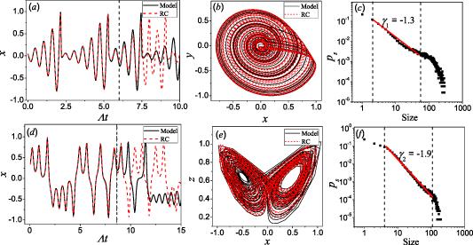
Figure 2. Results on chaotic system prediction and synchronization cluster size distribution using traditional RC. (a) The state prediction of the Rössler oscillator by RC. The black curve is obtained from numerical simulation of the real system. (b) The reconstruction of the Rössler attractor by RC. (c) The size distribution of the synchronization clusters in the predicting phase for RC. The result within $s\in[2, 60]$ are fitted by a power-law scaling $p^{s}\propto{s^{\gamma}}$, with $\gamma_{1}\approx-1.3$. (d) and (e) are the state prediction and attractor reconstruction for the Lorenz system by RC, respectively. (f) The size distribution of the synchronization clusters. The results within $s\in[4,100]$ are fitted by a power-law scaling $p^{s}\propto{s^{\gamma}}$, with $\gamma_{2}\approx -1.9$. |
Table 1. Hyperparameter sets of RC under different tasks and corresponding statistical parameter combinations for synchronization cluster statistics. RC$ _{\mathrm{g}}$ and RC$ _{\mathrm{b}}$ refer to examples with successful and failed training in the main text, respectively. MulRC2 and MulRC3 correspond to examples with two and three attractors memorized simultaneously by multifuntional RC, respectively. |
| Cases | d | σ | a | $\lambda$ | ξ | Statistical parameters |
|---|---|---|---|---|---|---|
| RC$ _{\mathrm{g}}$-Rössler | 0.4 | 1 | 0.3 | 1 | $1\times10^{-7}$ | $(\triangle{T}, p_\mathrm{c}, M)$ = (1000, 0.95, 500) |
| RC$ _{\mathrm{b}}$-Rössler | 0.1 | 0.1 | 0.1 | 1 | $1\times10^{-7}$ | $(\triangle{T}, p_\mathrm{c}, M)$ = (1000, 0.95, 500) |
| RC$ _{\mathrm{g}}$-Lorenz | 0.4 | 1 | 0.85 | 1 | $1\times10^{-7}$ | $(\triangle{T}, p_\mathrm{c}, M)$ = (150, 0.98, 500) |
| MulRC2-Rössler | 0.012 | 0.7 | 0.1 | 2.31 | $1\times10^{-8}$ | $(\triangle{T}, p_\mathrm{c}, M)$ = (1000, 0.95, 500) |
| MulRC2-Lorentz | 0.012 | 0.7 | 0.1 | 2.31 | $1\times10^{-8}$ | $(\triangle{T}, p_\mathrm{c}, M)$ = (150, 0.98, 500) |
| MulRC3-Chua's circuit | 0.42 | 0.6 | 0.97 | 2.5 | $1\times10^{-8}$ | $(\triangle{T}, p_\mathrm{c}, M)$ = (150, 0.98, 500) |
Initially, the neurons within the RC act as oscillators with randomized initial values and remain in a quiescent state. Upon being driven by external input signals (once the training process commences), the RC can be characterized as a dynamical system. Following successful training, the system begins autonomous evolution during the prediction phase. This process naturally raises two fundamental questions: (1) What are the properties of the internal neuronal states after the RC has successfully learned a predefined task? (2) If such properties exist, to what extent are they universal? In other words, when learning different tasks, does RC always exhibit similar characteristics? These questions are motivated by insights from neuroscience, where criticality has been established as a necessary condition for the brain's healthy functioning. Identifying analogous necessary conditions for the proper operation of machine learning systems would hold significant implications for the design and optimization. Therefore, we will analyze the collective behavior of the nodes within the RC from the perspective of synchronization patterns, which are calculated from the time series of the oscillators. Specifically, as shown in figure 1(b), in the prediction phase, a segment of equal length $\Delta{T}$ is first taken from each oscillator's time series across a common time window. These segments, labeled as data points $r_{i}(t_{0}+1),\ldots,r_{i}(t_{0}+\Delta{T})$ where $i, = 1,\ldots,D_\mathrm{r}$, are then used to compute all pairwise Pearson correlation coefficients. Among them, the time point t0 can be freely selected anywhere within the evolutionary sequence of the RC. A synchronous cluster is formed by grouping every pair of oscillators whose correlation surpasses a predefined threshold $p_\mathrm{c}$. The number of oscillators contained within each cluster represents the cluster size. Following this, the size distribution of the synchronous clusters can be calculated. It should be noted that a single RC of limited size ($D_\mathrm{r}$ = 2000) might be insufficient for generating a robust statistical distribution. Therefore, we employed an ensemble of M RC replicas, all sharing the same hyperparameters but constructed with different random seeds, which result in differences in $\boldsymbol{W}_{\textbf{in}}$ and A. Each replica was confirmed to perform proficiently in prediction tasks, including accurate short-term forecasting and attractor reconstruction. Ultimately, across these M replicas, the total number of clusters of size s is counted, and the corresponding distribution p(s) is computed accordingly (an approach known as ensemble averaging).
The statistical parameters for identifying synchronous clusters were set to $\Delta{T}$ = 1000, $p_\mathrm{c}$ = 0.95, and M = 500. Figure 2(c) displays the relationship between the distribution probability ps, defined as the probability of detecting a cluster of size s across the M RCs, and the cluster size s. The result indicates that the size distribution of synchronous clusters approximately follows a power-law scaling $p_{s}\propto{s^{\gamma}}$, with $\gamma_{1}\approx-1.3$, within the range of $s\in[2,60]$. It is necessary to provide a few detailed explanations of the fitting process. We employed the least squares method to fit the distribution for $s\in[s_\textrm{min}, s_\textrm{max}]$. Following established practices in neuroscience [44], we quantified the fitting error using a normalized distance $\hat{D} = \Sigma_{s}|p_{s}-p_{s}^\textrm{fit}|/\Sigma_{s}sp_{s}$, where $p_{s}^\textrm{fit}$ is the fitted probability of detecting a pattern of size s. Put simply, $\hat{D}$ measures the difference in the average synchronous cluster size between the actual evolution results of RC and the fitted results. Consequently, a smaller value of $\hat{D}$ indicates a superior fit. For the task of predicting Rössler oscillator, the values of $s_\textrm{min}$ = 2 and $s_\textrm{max}$ = 60 were chosen with the aim of minimizing the normalized distance $\hat{D}$. Small clusters are excluded from the analysis as they are prone to systemic fluctuations and noise and thus do not reliably represent the system's underlying statistical properties. This approach is consistent with established practices in neuroscience [45, 46].
The result in figure 2(c) suggests that the successfully trained RC exhibits critical-like behavior, akin to a normally functioning brain. To further validate this finding, we retrained the RC to predict the dynamics of another chaotic system, the Lorenz oscillator: $(\textrm{d}x/\textrm{d}t, \textrm{d}y/\textrm{d}t, \textrm{d}z/\textrm{d}t)^{\textrm{T}} = [10(y-x), 35x-y-xy, -8/3z+xy]^{\textrm{T}}$. The system exhibits chaos, with the largest Lyapunov exponent $\mathnormal{\Lambda}\approx1.03$. As shown in figures 2(d) and (e), the RC successfully predicts the time series for over 8 Lyapunov times and reconstructs the attractor. Calculation from $\tilde{T} = 6000$ data points (spanning more than 300 Lyapunov times) yields $D_{0} = 0.3$ and D = 0.32, pointing to its capability to replicate the Lorenz oscillator's 'climate'. The hyperparameters are shown in the RC$ _{\mathrm{g}}$-Lorenz row in table 1. As shown in figure 2(f), the size distribution of synchronization clusters adheres to a power law for sizes $s\in[4, 100]$, with a scaling exponent of $\gamma_{2}\approx-1.9$ (statistical parameters: $T = 150, p_\mathrm{c} = 0.98, M = 500$). This result is divergent from that in figure 2(c), demonstrating that the RC's internal statistical characteristics are task-dependent, yet consistently display power-law scaling.
When the brain is in an abnormal state, it often deviates from the critical state. Therefore, we cannot help but wonder what happens to a poorly trained RC. To illustrate this, we reset the hyperparameters (RC$ _{\mathrm{b}}$-Rössler in table 1) and train the RC with the same dataset used in figure 2(a). The reconstruction of the attractor is shown in figure 3(a), where it can be observed that the prediction completely fails. Here, we regard this machine as being poorly trained, and denote it by RC$ _{\mathrm{b}}$. The size distribution of the synchronous clusters is shown in figure 3(b). It deviates significantly from that of the successfully trained machine, denoted as RC$ _{\mathrm{g}}$, whose result is identical to that in figure 2(c).
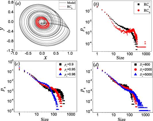
Figure 3. The prediction result from a poorly trained RC model (RC$ _{\mathrm{b}}$) and the effect of statistical parameters on size distribution for Rössler system. (a) The reconstruction of the Rössler attractor by RC$ _{\mathrm{b}}$. (b) The size distribution from the properly (RC$ _{\mathrm{g}}$) and poorly (RC$ _{\mathrm{b}}$) trained machines. (c) The size distributions for different values of $p_\mathrm{c}$. (d) The size distributions for different reservoir size ($D_\mathrm{r}$). |
The potential influence of statistical parameters on the distribution must be taken into consideration. Using the learning task for the Rössler oscillator as an example, we systematically evaluate the influence of three parameters on the distribution. First, with $\Delta{T}$ and M held constant, we varied $p_\mathrm{c}$. The results are shown in figure 3(c), which clearly demonstrate that the three outcomes are approximately identical when $s\in[2,30]$. The most significant discrepancies are evident in the distribution tails. Specifically, as $p_\mathrm{c}$ increases, the tail is shifted to the left slightly. The results is reasonable, as by increasing $p_\mathrm{c}$ the probability for generating larger-size clusters will be decreased. Here, setting $p_\mathrm{c}$ = 0.95 yields a better power-law distribution (i.e. a smaller $\hat{D}$) for the synchronous cluster size across a broader range compared to other threshold values. This reason motivates our selection of this specific threshold. We next examine the other two parameters by varying them within specific intervals, $\Delta{T}\in [1000,2000]$, $M\in[500,1000]$. The size distribution remained nearly unchanged across these variations (not shown). Moreover, the distribution showed little dependence on the specific position (i.e. the location of t0) of the segment ($\Delta{T}$), within the RC evolutionary sequence. These results suggest that once the RC has learned a task, its macroscopic statistical properties become relatively stable. Lastly, a discussion of the finite-size effects on the RC's distribution characteristics is also essential. We held all parameters except $D_\mathrm{r}$ constant, maintaining identical hyperparameters and statistical parameters to those used in figure 2(c). The reservoir was retrained on the Rössler oscillator with $D_\mathrm{r}$ values of 800, 2000, and 5000, and the size distributions of the synchronous clusters are presented in figure 3(d). As observed, the three distributions nearly overlap in the small-size region, with differences primarily evident in the tails. Moreover, a rightward shift in the distribution is apparent as the value of $D_\mathrm{r}$ increases.
3.2. The verification of critical-like behavior
In the aforementioned study, we employed the least squares method, incorporating a normalized distance $\hat{D}$ criterion, to fit the cluster size distribution and observed that the successfully trained RC exhibits critical-like behavior. Currently, another commonly adopted approach for fitting power-law distributions is the Kolmogorov-Smirnov (KS) statistical method [46], which is based on the cumulative distribution function (CDF). For any probability distribution P(x), it is given by
$equation$
For the CDF of real data derived from RC statistics, $C_{\mathrm{RC}}(s)$, and the fitted distribution, $C_{\mathrm{fit}}(s)$, the KS-statistic is defined as $equation$
Minimizing the objective function $D({\boldsymbol{x}};\gamma)$ yields an estimate for the slope parameter γ of the power law model $equation$
The distribution slopes for the Rössler and Lorenz systems were recalculated using the KS statistic, followed by a comparison with the least squares method in table 2, which also includes the fitting ranges for the real data under both methods. Furthermore, in the context of KS statistics, the p-value and the 95% confidence interval serve as key criteria for assessing the goodness-of-fit of a power-law distribution. Specifically, following the methodology of [46], we used a bootstrap approach with 1000 resamples to estimate the p-value (the p-value was defined as the fraction of synthetic KS distances exceeding the KS distance of the real data) and 95% confidence interval for the power-law exponent. The corresponding results are also listed in table 2. The reliability of the fitting procedure is substantiated by the combination of large p-values (generally exceeding 0.1) and tight confidence intervals.
Table 2. Comparing least squares (LS) and KS statistics for power-law fitting of size distributions in RC internal nodes across tasks. γ: fitting slope (scaling exponent). $[s_\textrm{min},s_\textrm{max}]$: fitting range. $\hat{D}$: normalized distance. |
| Methods | γ | $[s_\textrm{min},s_\textrm{max}]$ | $\hat{D}$ | p | 95% confidence interval |
|---|---|---|---|---|---|
| LS-Rössler | -1.3 | [2,60] | 0.11 | - | - |
| LS-Lorenz | -1.9 | [4100] | 0.13 | - | - |
| KS-Rössler | -1.313 | [2,55] | - | 0.752 | [-1.389, -1.237] |
| KS-Lorenz | -1.92 | [4108] | - | 0.857 | [-1.989, -1.851] |
Despite the slight discrepancy in the scaling exponent γ of the power-law fits between the two methods, as shown in table 2, our primary conclusion remains robust: learning different chaotic systems drives the internal nodes of the RC to self-organize into synchronous clusters with distinct distributional properties. This central claim is further substantiated by the multi-task learning results discussed below.
4. The results of multifunctional RC
Currently, predicting chaotic systems is a relatively simple task for RC. If more complex tasks are to be learned, what characteristics would emerge within RC? For this purpose, we built a multifunctional RC using equation (4 ) that was designed to simultaneously memorize m = 2 chaotic attractors, namely the Rössler and Lorenz attractors. To enable efficient memorization, following [29], we introduced a separation parameter η to process the input data (training data), with the goal of separating the m attractors in opposite directions in phase space, which, according to the studies in neuropsychology, is helpful for the storage and retrieval of multiple memories [41, 42]. Specifically, the states $(x,y,z)$ of the Rössler and Lorenz are replaced by $(x+\eta, y+\eta, z+\eta)$ and $(x-\eta, y-\eta, z-\eta)$, respectively, with η = 0.5. Furthermore, we set the labels $\beta_{1} = 0.1$ and $\beta_{2} = 0.2$ to the Rössler and Lorenz attractors, respectively. It is worth noting that the label value, β, may be freely selected within a suitable range, as this choice does not affect the learning outcomes of RC and the properties of the distribution. In the training data preparation stage, time series segments of length T = 3000 are collected from each attractor and normalized by their respective maximum values. These segments are concatenated into a single training set with a total length of $\hat{T} = 2T$, which is subsequently used as input to the machine for the computation of $\boldsymbol{W}_{\textbf{out}}$. The first τ reservoir states obtained after feeding each segment T into the machine are discarded. To obtain the optimal set of hyperparameters during the validation phase, the states of RC are first initialized with random values. The machine is then driven by the label βi to operate in the closed form. However, prior to fully autonomous phase, as previously mentioned, the RC is driven with l = 15 data points from the true attractor, which facilitates the successful retrieval of the target dynamics. Following τ steps of autonomous evolution, we collect $\tilde{T} = 6000$ output values for calculating the deviation Di. This operation is identically performed for each attractor. The objective function used in the search for the optimal hyperparameters is then defined as $\tilde{D} = \frac{\Sigma_{i = 1}^{m}|D_{i}-D_{0i}|}{m}$. The optimal hyperparameters are obtained after 1000 trials in the parameter space with the help of the 'optimoptions' function in MATLAB. The search ranges for the hyperparameters are $d\in(0,0.5], \sigma\in(0,1], \alpha\in(0,1], \lambda\in(0,3], \xi\in[1\times{10^{-8}},1\times{10^{-2}}]$. The hyperparameters are shown in the MulRC2-Rössler (MulRC2-Lorenz) row in table 1.
During the retrieval phase, attractor label βi (randomly selected from all labels) is input into the machine. The RC evolves from the arbitrary initial state, similar to the procedure in the validation phase, and is first driven by l = 15 data points sampled from the true attractor before transitioning to autonomous evolution. Throughout this process, $\tilde{T} = 6000$ data points are collected to compute the deviation metric Di. The retrieval is deemed successful if the condition $|D_{0i}-D_{i}|\unicode{x2A7D}{D_\mathrm{c}}$ is satisfied. Figure 4(a) presents that two attractors are successfully retrieved. The black and blue attractors are derived from the real system, while the red and green ones come from RC predictions. We proceed by holding the RC's hyperparameters constant, as outlined before, while repeatedly varying the random seed used during its construction. This training and retrieval cycle is repeated until M = 500 RC realizations capable of successfully retrieving all attractors are obtained. Throughout this process, we calculate the distribution of synchronous cluster sizes within the multifunctional RC. The specific statistical parameters used differ depending on which attractor is being retrieved. Specifically, when an attractor is retrieved, the statistical parameters applied are the same as those used for its prediction with traditional RC, i.e. $\Delta{T}$ = 1000, $p_\mathrm{c}$ = 0.95 for the Rössler attractor, and $\Delta{T}$ = 150, $p_\mathrm{c}$ = 0.98 for the Lorenz attractor. Regarding the size distributions within the multifunctional RC during retrieval of the Rössler and Lorenz attractors, these are shown in figures 4(b) and (c), respectively. For comparison, the corresponding results from the traditional RC, figures 2(c) and (f), are also included in the plots. We are surprised to find that when the multifunctional RC successfully retrieves a chaotic attractor, the size distribution of its synchronous clusters not only exhibits power-law scaling but also shows near-perfect agreement with the distribution generated by a traditional RC predicting that same attractor. This indicates that when a multifunctional RC memorizes multiple chaotic attractors, its internal nodes form stable and unique functional networks corresponding to each attractor. When retrieving different attractors, the functional networks switch autonomously. To verify this, we next configured the RC to memorize three chaotic attractors.
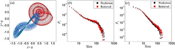
Figure 4. The retrieval results of two attractors and the synchronous cluster size distribution by the multifunctional RC. (a) Two attractors are accurately retrieved from the multifunctional RC. (b) The size distribution of the traditional RC for predicting the Rössler system (black) is compared with that of the multifunctional RC for retrieving the Rössler attractor (red). (c) Results for the Lorenz system. |
The third chaotic attractor is Chua's circuit, and its dynamic is described by: $(\textrm{d}x/\textrm{d}t, \textrm{d}y/\textrm{d}t, \textrm{d}z/\textrm{d}t)^{\textrm{T}} = [c_{1}(y-x-g(x)), c_{2}(x-y+z), -c_{3}y]^{\textrm{T}}$, with $g(x) = m_{1}x+(m_{0}-m_{1})(|x+1|-|x-1|)/2$. The system parameters are chosen as $(c_{1}, c_{2}, c_{3}, m_{0}, m_{1}) = (15.6, 1, 33, -8/7, -5/7)$, by which the system presents chaotic motion, with the largest Lyapunov exponent being about $\mathnormal{\Lambda}\approx0.92$. The states $(x,y,z)$ of Rössler, Lorenz and Chua's circuit are replaced by $(x+\eta, y+\eta, z+\eta)$, $(x-\eta, y-\eta, z-\eta)$ and $(x,y,z)$, respectively, with η = 0.2. The three attractors are assigned the labels $\beta_{1} = 0.1, \beta_{2} = 0.5$, and $\beta_{3} = 0.3$, respectively. The training and validation process was the same as that for the two attractors. For Chua's circuit, $D_{0} = 0.48$ and D = 0.52. The hyperparameters are shown in the MulRC3-Chua's circuit row in table 1, and T = 3000, $\hat{T} = 3T$. Figure 5 shows the size distributions of synchronous clusters during the retrieval of each of the three attractors by the multifunctional RC, revealing that distinct functional networks are formed within the RC for different memorized attractors.
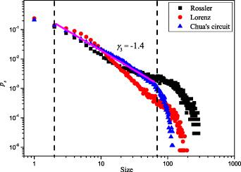


Figure 5. The size distribution of the multifunctional RC when successfully retrieving the three chaotic attractors. The distribution of Chua's circuit within $s\in[2,70]$ are fitted by a power-law scaling $p^{s}\propto{s^{\gamma}}$, with $\gamma_{3}\approx -1.4$. |
5. Conclusion and discussion
In recent years, the remarkable achievements of ANN across various fields have been astounding. But its mechanism remains unclear, which is why it is still called a black box. Part of the difficulty stems from the fact that these mechanisms may hinge on a multifaceted theoretical foundation. We begin from the theory of synchronization patterns in complex systems. As ANN is brain-inspired structures whose design and function mimic the brain, we wonder whether its statistical characteristics during operation also parallel neural activity. A widely accepted view posits that the normal brain functions at a self-organized critical state. Accordingly, we investigate the workings of machines through the same lens. In traditional RC, for instance, our studies show that successful training leads to the emergence of spontaneous synchronization clusters among internal nodes, with their size distribution exhibiting a clear power law, a key marker of criticality. Furthermore, the robustness of this distribution to changes in statistical parameters ($\Delta{T}, M, p_\mathrm{c}$) suggests that critical-like behavior is a stable characteristic maintained during RC evolution. The distribution characteristics, however, are task-dependent: the scaling law changes with the chaotic system being learned. By contrast, poorly trained RC yields no power-law signature. This initially suggests that learning distinct tasks imprints different traces on the RC, which may in turn be understood as the formation of task-specific functional networks within the RC. We validate this by designing a multifunctional RC. Once trained, it can retrieve the attractor associated with any input label βi through its parameter channel. Herein, the size distribution of synchronous clusters inside the multifunctional RC also exhibits a distinct power-law characteristic, and this distribution is almost identical to that when the traditional RC predicts the attractor independently. Subsequently, upon changing the input label value, the RC not only reconstructs a new attractor but also enables the autonomous switching of the size distribution of synchronous clusters.
In light of the present study, the following points are offered for open discussion. (1) Methods for identifying criticality in dynamical systems continue to evolve. A common criterion is the presence of scale-invariant macroscopic behavior, evidenced by power-law distributions with specific correlations in space and time. Complementary evidence may be drawn from finite-size scaling and spectral analysis. In this study, we observed spatial power-law behavior in a trained RC, though other criticality signatures remain unconfirmed. Hence, we describe the system as exhibiting critical-like behavior. Further work is needed to validate this phenomenon more rigorously. (2) The power-law exponents associated with these cluster distributions serve as characteristic 'fingerprints' that uniquely identify each attractor. This phenomenon may be attributed to the formation of distinct mapping relationships between the reservoir and various target systems during training, a process consistent with the establishment of generalized synchronization. Such relationships likely enable the learned information to be encoded within a complex ensemble of metastable states embedded in the reservoir's internal dynamics. When the system is driven by cues corresponding to different attractors, the reservoir's trajectory undergoes corresponding transitions, giving rise to distinct statistical properties at the macroscopic level. (3) Based on the current findings, critical-like behavior may be a necessary condition for RC to acquire knowledge. However, whether such behavior exhibits a well-defined boundary corresponding to RC performance, or whether it maps onto a specific region within the hyperparameter space, remains inconclusive-largely due to the computational challenges associated with exhaustive parameter scanning. Nevertheless, continued investigation holds promise for informing the future design of RC architectures and guiding hyperparameter optimization.