


1 Introduction
Quantum metrology aims to obtain the higher sensitivity in parameter estimation using quantum mechanics methods.[1-4] The physical quantities, e.g. gravitational waves, electric fields, weak magnetic fields, atomic frequencies, are generally transformed into phase shifts which can be accurately measured through interferometric experiments,[5] i.e., Mach-Zehnder interferometer (MZI). The phase sensitivity in linear optical MZI with classical approaches is limited by shot noise limit (SNL), i.e., $1/\sqrt{N}$, where $N$ is the average number of photons inside the interferometer. However, more works have shown that the use of entangled state like NOON state[6] can lead to improved sensitivity in optical-phase measurements. Restricted by Heisenberg's uncertain relationship, the improved sensitivity can beat the SNL and reaching the Heisenberg limit (HL), i.e., $1/N$.[7]
In 1981, Caves et al.[3] proposed a scheme in optical interferometry that the SNL can be beaten by using coherent $\otimes$ squeezed-vacuum light as input. This scheme has been used in gravitational wave detection experiments, for example GEO600[8] and LIGO.[9] In 1986, Yurke et al.[4] proposed another novel nonlinear interferometer, which replaced the 50:50 beam splitter in traditional MZI with active elements of optical parameter amplification (OPA) or four-wave mixing (FWM). They called this nonlinear interferometer as the SU(1,1) interferometer and the linear MZI as the SU(2) interferometer. A series of recent studies have shown that the SU(1,1) interferometer not only improves the phase measurement sensitivity compared with the SU(2) interferometer, but also performs more robust in suppressing detection noise.[10-12] Recently, Plick et al.[13] improved the original SU(1,1) interferometer. In their scheme, a strong coherent light beam was added, which solved the problem of the low number of photons of squeezed state prepared by the original scheme, and greatly improved the sensitivity of phase measurement. The SU(1,1) interferometer has been successfully implemented in the experiment.[14-15] Loss is one of the limit factors in parameter estimation. Recently, Mathieu Manceau et al.[10] showed that for a given gain of the first parametric amplifier, unbalancing the interferometer by increasing the gain of the second amplifier improves the interferometer properties. In this scheme, one can gain the optimal sensitivity even with the existence of external losses.
Recently, some researches on the phase sensitivity in SU(2) interferometry with two types of phase shift-one-arm and two-arm have been done.[16-17] The results showed different phase shifts have an important impact on the ultimate precision. Moreover, some relevant researches on one-arm[18-21] and two-arm[11,22-23] phase-accumulated SU(1,1) interferometer have been proposed. In Refs. [18--19], the authors discussed the achievable sensitivity with homodyne detection and showed it can approach HL for coherent and squeezed vacuum states. As is well known, the fundamental phase sensitivity is set by the quantum Cramér-Rao bound (QCRB). Does the homodyne detection can reach this sensitivity bound in the above scenario? This question has not yet been addressed in Refs. [18--19]. Meanwhile, for two-arm phase accumulating case, the fundamental phase sensitivity for a several of probe states was obtained in Refs. [22--23], while the discussion about the feasible detection method approaching such sensitivity was missed. In this paper, we make a full analysis of the phase sensitivities in one-arm and two-arm phase-shift accumulating SU(1,1) interferometer by using coherent $\otimes$ squeezed vacuum states, and then discuss the achievable sensitivities with the homodyne measurement. By analytically calculating the QFI, we find that the two-arm case shows a better precision with high strength of squeezed vacuum state, when compared with the single-arm case. However, such advantage does not take place in realistic measurement. To clarify this, we derive the achievable sensitivity with homodyne detection by invoking of error-propagation formula. Our results show that the achievable sensitivities are identical in both two phase shift cases. Although they approach HL, they can not saturate the QCRB. Due to photon losses and detector imperfections, the actual measurement sensitivities are often worse than the theoretical results. We further discuss the effects of photon losses on the achievable sensitivities for the two phase shift cases. We finally find that the unbalanced interferometer helps to improve precision for both cases even with high external losses.
This paper is organized as follows. In Sec. 2, we first briefly introduce the standard SU(1,1) interferometer and compute the theoretical phase sensitivities with the different types of phase shift. In. Sec. 3, we explicitly derive the ultimate phase sensitivities by homodyne detection. Moreover, in Sec. 4, we specifically study the SU(1,1) interferometer in the presence of detection noise and internal losses. Finally, the conclusions are given in Sec. 5.
2 The SU(1,1) Interferometer with Two Different Phase Shifts
$$ a_{1} = a_{0}\text{{cosh}}s_{1}-{{\rm i}e^{{\rm i}\vartheta_{1}}}b_{0}^{\dagger}\sinh s_{1}\,,\\ b_{1} = b_{0}\text{{cosh}}s_{1}-{{\rm i}e^{{\rm i}\vartheta_{1}}}a_{0}^{\dagger}\sinh s_{1}\,, $$
where $s_{1}$ and $\theta_{1}$ describe the gain factor and phase of the first OPA. $a_{0} \,(a_{0}^{\dagger}$) and $b_{0}\,(b_{0}^{\dagger}$) are the annihilation (creation) operators of the upper and lower input modes of the interferometer, respectively.
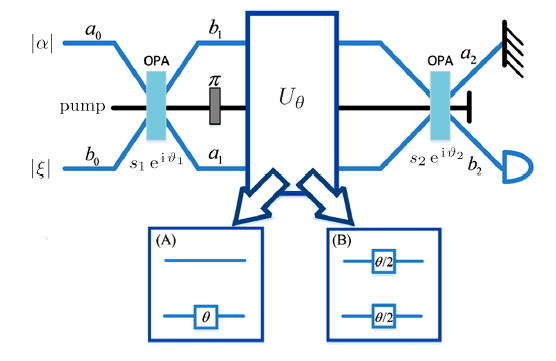
Fig. 1 (Color online) SU(1,1) interferometer model with two types of phase shift: one-arm and two-arm. The input state is $|\alpha\rangle\otimes|\xi\rangle$. After the first OPA, it accumulates an unknown phase, which is determinated by $U_{\theta}$. Then it goes through the second OPA and a homodyne measurement is performed. The pump field between the two OPAs has a $\pi$ phase difference. |
Let $|\psi_{{\rm in}}\rangle$ denote the state entering at the input ports of the interferometer. Here we use coherent $\otimes$ squeezed vacuum states, i.e., $|\alpha\rangle\otimes|\xi\rangle$ as probe state, where $\alpha=|\alpha|{e^{{\rm i}\vartheta_{\alpha}}}$ and $\xi=r{e^{{\rm i}\vartheta_{\xi}}}$. The phase shift can be expressed by unitary operator $U_{\theta}=\exp({-{\rm i}\theta H})$, where $H$ denotes the Hermitian generator. In this article, we consider two cases of phase shift operation acting on: (i) One arm, i.e., $H=a^{\dagger}a$ and (ii) both arms, i.e., $H=(a^{\dagger}a+b^{\dagger}b)/2$. Then the state at the output ports reads $|\psi_{{\rm out}}\rangle={{\rm OPA}}_{2}U_{{\theta}}{{\rm OPA}}_{1}|\psi_{{\rm in}}\rangle$.
Theoretically, the phase measurement sensitivity is limited by the quantum Cramér-Rao bound (QCRB), which is one of the most important quantities for both quantum estimation theory and quantum information theory, has been widely studied.[1-2,24] The lower bound of the QCRB is provided by the inverse of quantum Fisher information (QFI), which depends only on the probe state and phase accumulation. Regardless of the measurement part, the theoretical sensitivity according to the quantum Cramér-Rao theorem satisfies the following inequality
$$ \Delta\theta_{{QCRB}}\geq\frac{1}{\sqrt{\upsilon F}}\,, $$
where $F$ represents the QFI and $\upsilon$ is the times of experiment operations.[1-2,{24}] Generally, such a bound can be reached by the maximum likelihood estimator for sufficiently large $\upsilon$ with Bayesian estimation methods.
For pure states $|\psi\rangle$, the QFI of the phase-dependent state $U_{{\theta}}|\psi\rangle$ can be represented as $F=4\langle(\Delta H)^{2}\rangle,$ where $(\Delta H)^{2}=\langle H^{2}\rangle -\langle H\rangle ^{2}$ with averaging over $|\psi\rangle$. In our cases, the QFIs under different phase shift procedures are given
$$ F_{{\rm A}} = 4|\alpha|^{2}\text{cosh}^{4}s_{1}+2\sinh^{2}2r\sinh^{4}s_{1}+\mathfrak{F}\,, $$
$$ F_{{\rm B}} = \Big(|\alpha|^{2}+\frac{1}{2}\sinh^{2}2r\Big)\text{cosh}^{2}2s_{1}+\mathfrak{F}\,, $$
where $\mathfrak{F}=(|\alpha|^{2}{e^{2r}}+\cosh^{2}r)\sinh^{2}2s_{1}$ and we have derived the optimal phase condition $2\vartheta_{1}-2\vartheta_{\alpha}-\vartheta_{\xi}=0$
under which the QFI get the maximum. Note that such an optimal phase condition is consistent with the phase-matching condition derived by Ref. [23].For simplicity, we set $\vartheta_{1}=\vartheta_{\alpha}=\vartheta_{\xi}=0$ in the following.
The mean photons on each arm are given by $n_{i}=\langle{n_{i}}\rangle$ ($i=a,b$). Note that ${n_{{ a}}}=|\alpha|^{2}$ and ${n_{{ b}}}=\sinh^{2}r$, so the total photon number of input state is $N_{0}={n_{{ a}}}+{n_{{ b}}}$. Due to the nonlinear property of OPA, the total number of photons after the ${{\rm OPA}}_{1}$ is enlarged as
$$ N_{{t}}=({n_{{a}}}+{n_{{b}}})\cosh2s_{1}+2\sinh^{2}s_{1}\,. $$
One can rewrite the expressions of Eqs. (3) and (4) in terms of ${n_{{ a}}}$ and ${n_{{ b}}}$. For given fixed $s_{1}$, $F/N_{{ t}}^{2}$ is plotted in Fig. 2. The green dashed line corresponds to the so-called "HL'', i.e., $\Delta\theta_{{HL}}=1/N_{{ t}},$ which is however not fundamental sensitivity limit when the particle number fluctuating presents.[{25-28}] From Fig. 2, one can see the amount of the QFIs become higher as the ${n_{{ b}}}$ increases for a fixed $N_{0}$. In the other words, one can get higher phase sensitivity by input a squeezed vacuum state with larger strength.
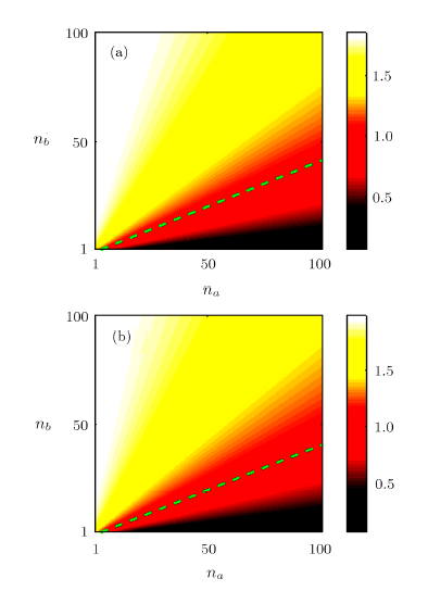
Fig. 2 (Color online) The variation of $F/N_{{ t}}^{2}$ as the function of $n_{{ a}}$ and $n_{{ b}}$ for phase shift in (a) one-arm and (b) two-arms. The gain factor of ${{\rm OPA}}_{1}$ is $s_{1}=2$. |
Next, we compare the theoretical sensitivities for both two types of phase shift according to Eq. (2). The difference of $\Delta\theta_{{QCRB}}^{{\rm A}}\sqrt{N_{{ t}}}-\Delta\theta_{{QCRB}}^{{Θ B}}\sqrt{N_{{ t}}}$ given by Eqs. (3) and (4) is plotted in Fig. 3(a), as a function of $n_{{ a}}$ and $n_{{ b}}$ with the gain factor $s_{1}=1$. The green dashed line represents the two sensitivities are identical. It is shown that the case with phase shift in both arms performs the better sensitivity when the strength of squeezed vacuum state is large enough.
A special case is considered here, we assume that $r=0$. As shown in Fig. 3(b), the ultimate sensitivities $\Delta\theta_{{QCRB}}\sqrt{N_{{ t}}}$, as a function of strength of coherent state $|\alpha|$, show that the phase shift in one arm can achieve the better sensitivity in this case.
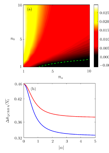
Fig. 3 (Color online) (a) Difference between the sensitivities of the two types of phase shift: $\Delta\theta_{{QCRB}}^{{A}}\sqrt{N_{{ t}}}-\Delta\theta_{{QCRB}}^{{B}}\sqrt{N_{{ t}}}$. The green dashed line represents the amount of QFIs in two cases is equal. (b) Phase sensitivity $\Delta\theta_{{QCRB}}\sqrt{N_{{ t}}}$ as a function of coherent amplitude $|\alpha|$ for $r=0$. The blue line is phase shift in one arm, the red line is phase shift in both arms. The gain factor of OPA$_{1}$ is $s_{1}=1$. |
3 Achievable Sensitivities by Homodyne Measurement
In this section, we discuss the measurement sensitivity achieved with typical measurement in two types of phase shifts. In general, the phase measurement uncertainty is still retrieved from a simplified error propagation theory, such that
$$ \Delta\theta=\frac{\Delta X}{\sqrt{\upsilon}|{\partial\langle X\rangle }/{\partial\theta}|}\,, $$
where $\langle X\rangle $ denotes the mean value of observable $X$ and $\Delta X=\sqrt{\langle X^{2}\rangle -\langle X\rangle ^{2}}$ is the root-mean-square fluctuation. In our scheme, we perform a homodyne detection on the output $b_{2}$,
$$ X(\phi) = \frac{1}{2}(b_{2}+b_{2}^{\dagger})\,. $$
3.1 Phase Shift In One Arm
We start with phase shift only in the lower arm. As depicted in Fig. 1, homodyne measurement is made on the port $b_{2}$. In this way the total transformation of input-output relations of the interferometer can be described by
$$ a_{2} =\mu a_{0}-{{\rm i}}\nu b_{0}^{\dagger}\,, $$
$$ b_{2} ={e^{{\rm i}\theta}}(\mu b_{0}-{{\rm i}}\nu a_{0}^{\dagger})\,, $$
where
$ \mu=\text{{cosh}}s_{1}\text{{cosh}}s_{2}{e^{-{\rm i}\theta}}+\sinh s_{1}\sinh s_{2}{e^{{\rm i}(\vartheta_{2}-\vartheta_{1})}}\,,\\\ \nu=\sinh s_{1}\text{{cosh}}s_{2}{e^{{\rm i}\vartheta_{1}}e^{-{\rm i}\theta}}+\text{{cosh}}s_{1}\sinh s_{2}{e^{{\rm i}\vartheta_{2}}}\,,$
such that $|\mu|^{2}-|\nu|^{2}=1$.
The SU(1,1) interferometer is typically studied in a balanced configuration in which the second parametric process is set to "undo''what the first parametric process did. Here, we first consider the balanced SU(1,1) interferometer configuration (i.e., $s_{1}=s_{2}=s$).To satisfy the optimal phase condition given previously, we also set $\vartheta_{\alpha}=\vartheta_{\xi}=\vartheta_{1}=0$. According to Ref. [19], when the phase of the second OPA $\vartheta_{2}=\pi$ may provide the maximal achievable sensitivity. Therefore the mean value $\langle X_{{ A}}\rangle $ and the expectation of $X_{{ A}}^{2}$ are given by respectively,
$$ \langle X_{{ A}}\rangle=-|\alpha|\sinh scoshs \sin θ $$
$$ \langle X_{{ A}}^{2}\rangle= \frac{1}{4}\Big[-\cos2\theta\Big(\sinh2r\sinh^{4}s+\frac{1}{2}|\alpha|^{2}\sinh^{2}2s\Big) \hphantom{\langle X_{{ A}}^{2}\rangle=} - \frac{1}{2}\sinh^{2}2s\cos\theta({e^{-2r}}+1)+\text{{cosh}}^{4}s({e^{-2r}}-1)^{2} \hphantom{\langle X_{{ A}}^{2}\rangle=} + \sinh^{2}2s\Big(\frac{1}{2}|\alpha|^{2}+1\Big)+2\sinh^{2}r\sinh^{4}s+1\Big]\,. $$
Submitting Eqs. (10) and (11) into Eq. (6) yields
$$ \Delta\theta^{{A}} = \frac{\sqrt{\langle X_{{ A}}^{2}\rangle -(|\alpha|\text{{cosh}}s\sinh s\sin\theta)^{2}}}{||\alpha|\text{{cosh}}s\sinh s\cos\theta|}\,. $$
To approach the "HL'', we need to find the optimal condition of the photon numbers at the input of the SU(1,1) interferometer. In the asymptotic limit $\theta\rightarrow0$, $\Delta\theta^{{A}}$ reduces to
$$ \Delta\theta^{{Θ A}}|_{\theta\rightarrow0}=\frac{1}{|\alpha|{e^{r}}\sinh(2s)}\,. $$
By using the relationships of ${n_{{ a}}}=|\alpha|^{2}$ and ${n_{{ b}}}=\sinh^{2}r$, one can rewrite this expression in terms of ${n_{{ a}}}$ and ${n_{{ b}}}$. Figure 4 is plotted by $N_{{ t}}\Delta\theta^{{A}}|_{\theta\rightarrow0}$ corresponding to ${n_{{ a}}}$ and ${n_{{ b}}}$ from $0$ to $100$. Similar to the MZI,[{29}] the photon numbers in two input ports of the SU(1,1) interferometer also need to balance to approach the optimal sensitivity.[19]
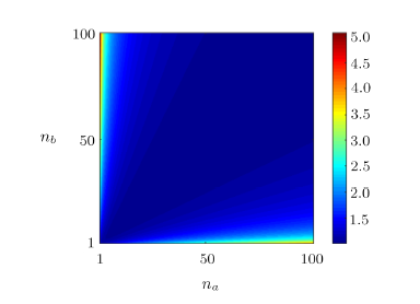
Fig. 4 (Color online) The sensitivity $N_{{ t}}\Delta\theta^{{A}}|_{\theta\rightarrow0}$ as a function of ${n_{{ a}}}$ and ${n_{{ b}}}$ with coherent state and squeezed vacuum state as the input state.$N_{{t}}$ is the total photons throughout the model. |
Figure 5(a) is plotted by Eq. (12) to show the ultimate sensitivity with phase shift in the lower arm.
As discussed above, the photon numbers of two input states need to balance, i.e., $|\alpha|=\sinh r$. As shown in the figure,the minimum of phase sensitivity occurs at $\theta=0$, given by Eq. (13). One can see this sensitivity in a range beats SNL far and approaches HL, which shows the same performance as discussed in Ref. [19]. In addition, we compare this result with the QCRB discussed in Sec. 2. We find it is close to QCRB at the optimal point, which means homodyne detection is a sub-optimal measurement in this case.
3.2 Phase Shift In Both Arms
Below we consider the case of phase shift in both arms, which is missed in Ref. [22]. In that case, the QFI for coherent and squeezed states was chiefly calculated. Similar to the previous process, we first get the total transform
$$ \tilde{a}_{2} =\tilde{\mu}a_{0}-{{\rm i}}\tilde{\nu}b_{0}^{\dagger}\,, $$
$$ \tilde{b}_{2} =\tilde{\mu}b_{0}-{{\rm i}}\tilde{\nu}a_{0}^{\dagger}\,, $$
where
$ \tilde{\mu}=\text{{cosh}}s_{1}\text{{cosh}}s_{2}{e^{-{\rm i}\theta/2}}+\sinh s_{1}\sinh s_{2}{e^{{\rm i}(\vartheta_{2}-\vartheta_{1})}e^{{\rm i}\theta/2}}\,,\\ \tilde{\nu}=\sinh s_{1}\text{{cosh}}s_{2}{e^{{\rm i}\vartheta_{1}}e^{-{\rm i}\theta/2}}+\text{{cosh}}s_{1}\sinh s_{2}{e^{{\rm i}\vartheta_{2}}e^{{\rm i}\theta/2}}\,.$
The phase matching condition is still the $\vartheta_{\alpha}=\vartheta_{\xi}=\vartheta_{1}=0$. We similarly consider the balanced case ($s_{1}=s_{2}=s$ and $\theta_{2}=\pi$). Using the same approach as in case A, the ultimate sensitivity is given by,
$$ \Delta\theta^{{Θ B}}=\frac{\sqrt{\langle X_{{ B}}^{2}\rangle -(|\alpha|\sinh(2s)\sin({\theta}/{2}))^{2}}}{||\alpha|\sinh s\text{{cosh}}s\cos({\theta}/{2})|}\,, $$
where
$$ \langle X_{{ B}}^{2}\rangle =-\frac{1}{4}\cos\theta\Big[\sinh^{2}2s \Big(2|\alpha|^{2}+\sinh^{2}r \hphantom{\langle X_{{ B}}^{2}\rangle}=+\frac{1}{2}\sinh2r+1\Big)+\sinh2r\Big]+\frac{1}{4}(2\sinh^{2}r+1) \hphantom{\langle X_{{ B}}^{2}\rangle =} +\frac{1}{4}\Big(2|\alpha|^{2}+\sinh^{2}r+\frac{1}{2}\sinh2r+1\Big)\,. $$
In the same way, we study the relation between two input ports photon numbers. When $\theta=0$, Eq. (16) reduces to
$$ \Delta\theta^{{B}}|_{\theta\rightarrow0}=\frac{1}{|\alpha|{e^{r}}\sinh(2s)}\,. $$
Interestingly, the optimal sensitivity is still obtained under the condition of ${n_{{ a}}}={n_{{ b}}}$,which satisfies with that in single-arm phase shift case.
Figure 5(b) shows the Eq. (16) as a function of $\theta$. These results are very similar to the ones calculated for case A. $\theta=0$ is still the optimal condition to achieve the ultimate sensitivity and likewise homodyne detection is still sub-optimal in this case. However, one can see the sensitivity is lower when $\theta$ is away from zero point.
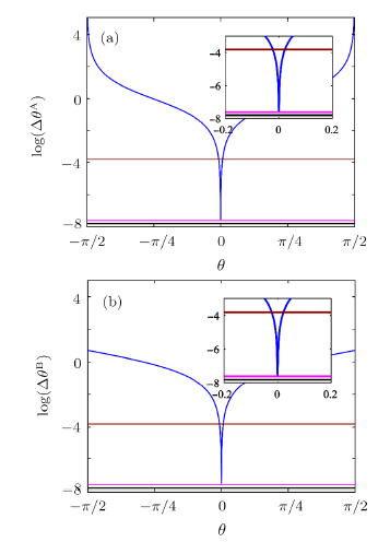
Fig. 5 (Color online) Log-plots of the phase sensitivities $\Delta\theta^{{A}}$ and $\Delta\theta^{{Θ B}}$ for both two cases with homodyne measurement (blue line), Eqs. (12) and (16),as a function of $\theta$. The strength of two OPAs is $s=2$. The parameters of input state are as follows: $r=2.5$, $|\alpha|=\sinh r$. |
The SNL is gray line and HL is purple line. The QCRB is presented by black line.
4 Effects of Experimental Noises and Unbalanced Scheme
As has been previously pointed out, the phase sensitivity is extremely affected by the photon losses both inside and outside of the interferometer due to the imperfections in the device and defects in the detector. We now turn to the effect of both of two types of losses on the measurement sensitivity in our scheme. Traditionally, photon losses can be modeled by adding an imaginary beam splitter and part of photons are dissipated into the environment when photons pass through, which can be described by
$$ a_{\rm out} = \sqrt{T_{i}}a_{\rm in}+\sqrt{1-T_{i}}c_{a}\,,\\\ b_{\rm out} = \sqrt{T_{i}}b_{\rm in}+\sqrt{1-T_{i}}c_{b}\,, $$
where $T_{i}$ is the efficiency of imaginary beam splitters. As shown in Fig. 6, $T_{1}$ and $T_{2}$ represent the transmission rates in presence of the internal and external losses respectively. $c_{a}$ and $c_{b}$ are the annihilation operators of the upper and lower loss modes of the interferometer. Here, we consider losses in both arms and continue to use coherent$\otimes$squeezed vacuum states as input state. Below, we detailly discuss the phase sensitivities achieved by the homodyne detection in the presence of both inside and outside losses separately.
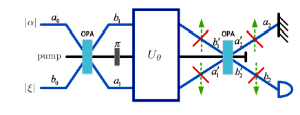
Fig. 6 (Color online) The loss model of SU(1,1) interferometer with homodyne measurement.The internal and external loss can be modeled by imaginary beam splitters. |
4.1 Phase Shift In One Arm
First, we discuss the sensitivity with phase shift in the lower arm under condition of $s_{1}=s_{2}=s$. Then the ultimate sensitivity with homodyne measurement is given by,
$$ \Delta\theta_{{L}}^{{A}}=\sqrt{(\Delta\theta^{{A}})^{2}+\frac{[T_{2}(1-T_{1})\cosh2s+1-T_{2}]}{T_{1}T_{2}|\alpha|^{2}\sinh^{2}(2s)\cos^{2}\theta}}\,, $$
which is composed of two parts, the first term is the ideal lossless sensitivity given by Eq. (12) and the second is the extra term due to the internal and external losses. When $T_{1}$ and $T_{2}$ equal to 1, the second term vanishes, and the sensitivity in this case will reduce to the ideal lossless case.
Figures 7(a) and 7(b) show the phase sensitivity $\Delta\theta_{{ L}}^{{A}}$ given by Eq. (20) in a narrow range close to $0$. In Fig. 7(a), we study the effect of internal losses on the interferometer by setting $T_{2}=1$ (no external losses). As can be seen from this figure, the increase of internal losses degrades the phase sensitivity. When $T_{1}=0.5$, it is impossible to beat the SNL. As shown in Fig. 7(b), it shows that the effect of the detection efficiency by making $T_{1}=1$. Compared to Fig. 7(a), one can see that SU(1,1) interferometer with phase shift in one arm shows the better performance in external noise resistance.
Now we study the unbalanced interferometer ($s_{1}\neq s_{2}$) with the existence of internal and external losses. The optimal condition $\theta=0$ is considered here. Under this condition, the phase sensitivity is given by
$$ (\Delta\theta_{{UL}}^{{{A}}})^{2} =\frac{1}{4|\alpha|^{2}\cosh^{2}s_{1}\sinh^{2}s_{2}} \Big[\mu^{2}{e^{-2r}}+\mu^{2} -1+\frac{T_{2}(1-T_{1})\cosh2s_{2}+1-T_{2}}{T_{1}T_{2}}\Big]\,, $$
where $\mu=\cosh s_{1}\cosh s_{2}-\sinh s_{1}\sinh s_{2}$.
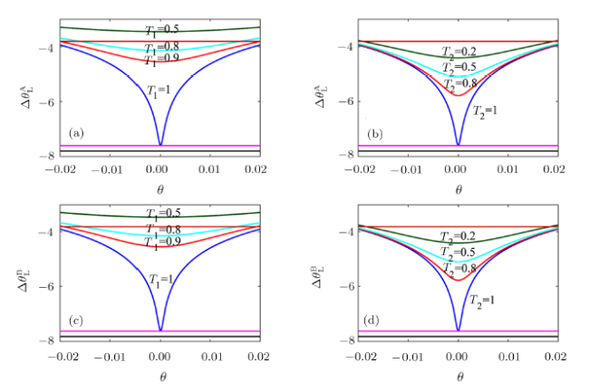
Fig. 7 (Color online) Log-plots of phase sensitivities with the existence of internal loss and external loss. (a), (b) Phase sensitivity $\Delta\theta_{{L}}^{{{A}}}$ as a function of $\theta$ in one-arm case. Different color curves represent different values of $T_{1}$ or $T_{2}$. (c), (d) Phase sensitivity $\Delta\theta_{{L}}^{{{B}}}$ as a function of $\theta$ in two-arm case. The SNL is gray line and HL is purple line. The QCRB is presented by black line. The parameters are as follows: $s=2$, $r=2.5$ and $\alpha=\sinh r$. |
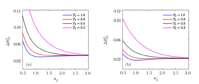
We keep the parameters of $T_{1}$ and $s_{1}$ unchanged and study the effect of $s_{2}$ on the ultimate sensitivity. Figure 8(a) shows the phase sensitivity $\Delta\theta_{{UL}}^{{{A}}}$ given by Eq. (21), as a function of $s_{2}$ for different values of $T_{2}$. It is confirmed that an increase of the second gain factor is helpful to improve precision even with high external losses and the ultimate sensitivity is close to ideal case. Similar results have been observed in Ref. [10].
4.2 Phase Shift In Both Arms
Next, we investigate the loss SU(1,1) interferometer with phase shift in both arms. Using the same approach as above, the ultimate sensitivity is given by:
$$ {\Delta\theta_{ {L}}^{ {B}}=\sqrt{(\Delta \theta^{ {B}})^{2}+\frac{[T_{2}(1-T_{1})\cosh 2s+1-T_{2}]}{T_{1}T_{2}|\alpha|^{2}\sinh^{2}(2s)\thinspace\cos^{2}({\theta}/{2})}}\,.} $$
As was done before, we separately consider the effect of internal losses and external losses on phase sensitivity in this case. The extra term is very similar to the one calculated for case A. Figures 7(c) and 7(d) are plotted by Eq. (22). As shown in the figure, the phase sensitivities achieved in both cases have the similar performance in noise resistance.
Finally, unbalanced interferometer is considered to study the influence of gain factor $s_{2}$ on the phase sensitivity with internal and external losses. In this case, the phase sensitivity is given by
$$ (\Delta\theta_{{UL}}^{Θ B})^{2} =\frac{1}{|\alpha|^{2}(\sinh s_{1}\cosh s_{2}+\cosh s_{1}\sinh s_{2})^{2}} \Big[\mu^{2} -1+\mu^{2}{e^{-2r}}+\frac{T_{2}(1-T_{1})\cosh2s_{2}+1-T_{2}}{T_{1}T_{2}}\Big]\,, $$
where $\mu=\cosh s_{1}\cosh s_{2}-\sinh s_{1}\sinh s_{2}$.
Figure 8(b) shows Eq. (23) as a function of $s_{2}$, and the result is much similar to the ones calculated for case A. When we introduce noise, an unbalanced interferometer model is good at resisting external loss. No matter what cases of phase shift, an increase of second gain factor $s_{2}$ will improve the ultimate sensitivity and finally eliminate the interference of external loss.
Fig. 8 (Color online) Phase sensitivities (a) $\Delta\theta_{{UL}}^{{{A}}}$ and (b) $\Delta\theta_{{UL}}^{{{B}}}$ as a function of gain factor $s_{2}$ for various values of the detection efficiency $T_{2}$ in unbalanced SU(1,1) interferometer. The parameters of input state are as follows: $r=3$, $\alpha=\sinh r$. Note that $s_{1}=1$ and $T_{1}=0.9$. |
5 Conclusion
In conclusion, we have studied the phase sensitivities of the SU(1,1) interferometer with two types of phase shift: One-arm and two-arms. For both two cases, we first exactly calculated the theoretical sensitivities for a mixing coherent state and squeezed vacuum state. We found that the sensitivity for two-arm phase shift case may outperform the single-arm case. We also considered the achievable sensitivity with homodyne measurement based on error propagation theory. Interestingly, we found that the achievable sensitivities for the two types of phase shift configuration provide the same sensitivity. It indicates that the advantage of sensitivity enhancement demonstrated above does not occur within practical measurement. Besides, we also showed that the homodyne detection is a sub-optimal measurement which can not saturate the QCRB but approach the HL. Finally, we considered effects of photon losses on the sensitivity of the SU(1,1) interferometer. We found that the achievable sensitivity degrades substantially when the internal and external losses exit. More importantly, in the unbalanced SU(1,1) interferometer, an increase of the gain of second OPA is helpful to resist and even eliminate the external loss for both two phase shift scenarios.
Note added Recently, Ref. [23] appeared, which derived a general phase-matching condition for maximal QFI in SU(1,1) interferometers for certain states, such as, coherent and even coherent states, squeezed vacuum and even coherent states, squeezed thermal and even coherent states. In this paper, we consider a different case by injecting a mixing of coherent state and squeezed vacuum state. The previous obtained phase-matching condition is also hold in our case, which can be complementary to applications in Ref. [23]. Our results on maximal QFI for two different phase shift configurations and phase sensitivities accessible by homodyne measurement with and without noises, however, are not covered in Ref. [23].