


1. Introduction
2. Preliminary definitions
The Caputo derivative
The FD and its Laplace transform (LT)
3. Model of the fractional order four-wing attractor, and its properties
3.1. Existence and uniqueness
if the nonlinear part, $F$, of system (8) satisfies the Lipschitz condition $\parallel F\left(u\right)-F\left(v\right)\parallel \leqslant \gamma \parallel u-v\parallel ,$ $\forall u,v\,\in {\Re }^{3},$ locally, in the presenec of a positive scalar, $\gamma \gt 0$, then system (8) has a unique solution [27].
Equilibrium points and eigenvalues
Bifurcation and Poincaré maps
Lyapunov exponents and the Kaplan-Yorke dimension
4. Simulation and results
4.1. Mathematical simulation
Table 1. Equilibrium point of system (8) at $a=1.5.$ |
| Points | $\alpha =1.00$ | $\alpha =0.99$ | $a=0.92$ | $a=0.90$ |
|---|---|---|---|---|
| ${P}_{0}$ | (0.,0.,0.) | (0.000 66,0.000 98,−0.001 00) | (0.005 02,0.007 36,−0.008 65) | (0.006 18,0.009 02,−0.011 04) |
| ${P}_{1}$ | (1.126 69,1.224 74,1.379 91) | (1.125 08,1.222 75,1.388 58) | (1.111 26,1.206 51,1.448 63) | (1.106 47,1.201 13,1.465 58) |
| ${P}_{2}$ | (1.126 69,−1.224 74,−1.379 91) | (1.1248,−1.221 86,−1.389 24) | (1.108 74,−1.199 29,−1.454 02) | (1.103 23,−1.192 07,−1.472 37) |
| ${P}_{3}$ | (−1.126 69,1.224 74,−1.379 91) | (−1.124 23,1.222 58,−1.389 35) | (−1.104 29,1.2048,−1.454 83) | (−1.097 71,1.198 87,−1.473 34) |
| ${P}_{4}$ | (−1.126 69,−1.224 74,1.379 91) | (−1.125 95,−1.223 46,1.390 47) | (−1.117 77,−1.211 96,1.4638) | (−1.114 47,−1.207 85,1.484 58) |
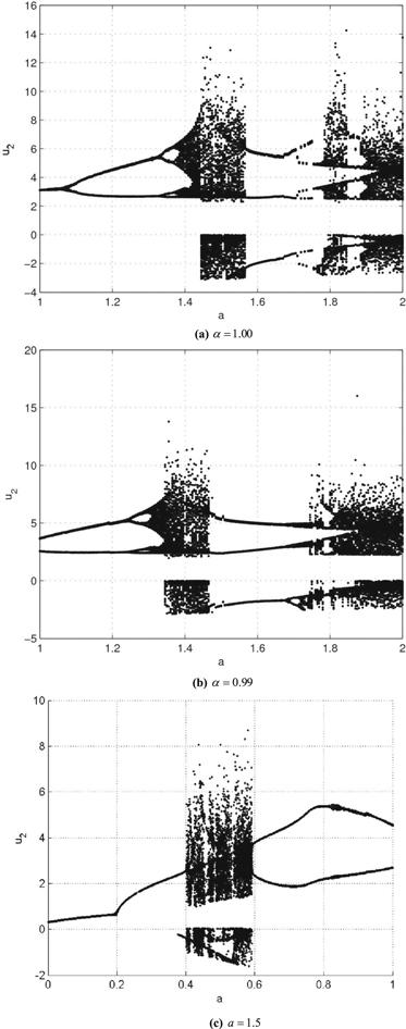
Figure 1. Bifurcation maps of system (8) for different parameters. |
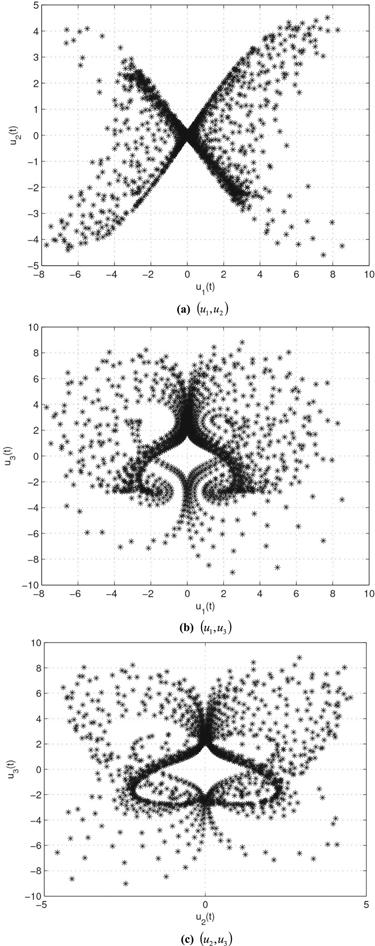
Figure 2. Poincaré section of system (8) at $\alpha =0.99.$ |

Figure 3. Plot ${u}_{1}\left(t\right)$ of system (8) for different values of $\alpha .$ |
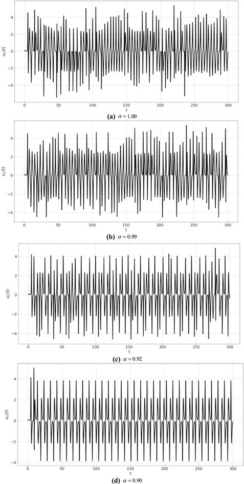
Figure 4. Plot ${u}_{2}\left(t\right)$ of system (8) at different values of $\alpha .$ |
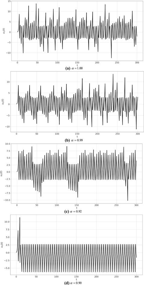
Figure 5. Plot ${u}_{3}\left(t\right)$ of system (8) for different values of $\alpha .$ |
Table 2. LE and KYD vakues for system (8). |
| $\alpha $ | ${L}_{1}$ | ${L}_{2}$ | ${L}_{3}$ | ${D}_{KY}$ |
|---|---|---|---|---|
| 1.00 | 0.266 697 | −0.017 213 | −4.695 504 | 2.053 13 |
| 0.99 | 0.273 420 | −0.017 020 | −4.804 732 | 2.053 36 |
| 0.92 | 0.003 342 | −0.267 246 | −3.945 491 | 1.933 11 |
| 0.90 | 0.000 167 | −0.303 911 | −3.942 772 | 1.922 96 |
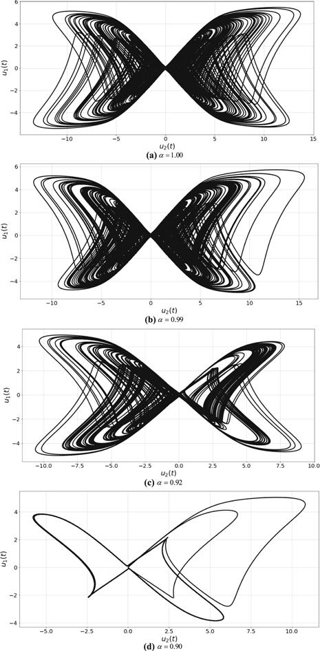
Figure 6. 2D phase plot (${u}_{1},{u}_{2}$) of system (8) for different values of $\alpha .$ |

Figure 7. 2D phase plot (${u}_{1},{u}_{3}$) of system (8) for different values of $\alpha .$ |
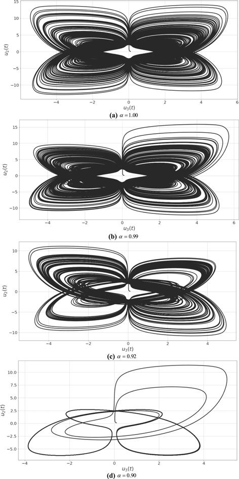
Figure 8. 2D phase plot (${u}_{2},{u}_{3}$) of system (8) for different values of $\alpha .$ |
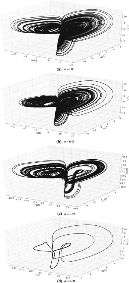
Figure 9. 3D flows of system (8) for different values of $\alpha .$ |
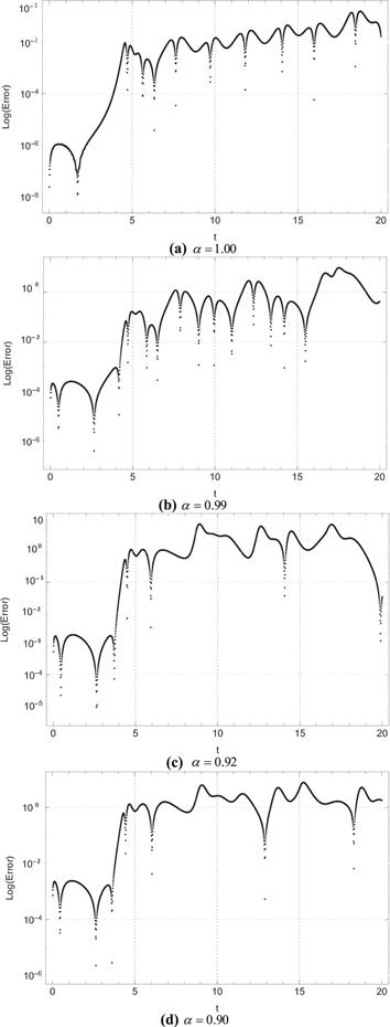
Figure 10. Log errors for ${u}_{1}\left(t\right)$ between system (1) and system (8). |
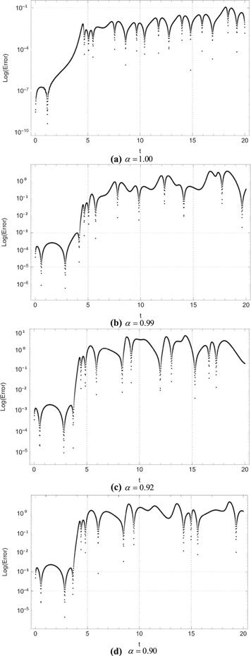
Figure 11. Log errors for ${u}_{2}\left(t\right)$ between system (1) and system (8). |
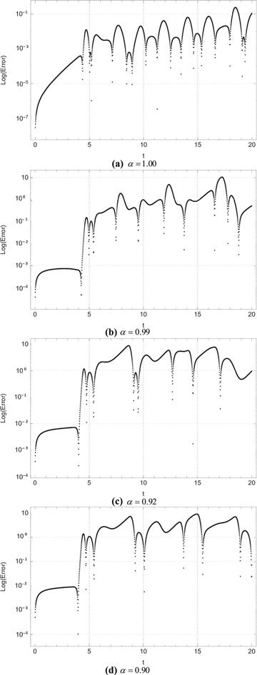
Figure 12. Log errors for ${u}_{3}\left(t\right)$ between system (1) and system (8). |
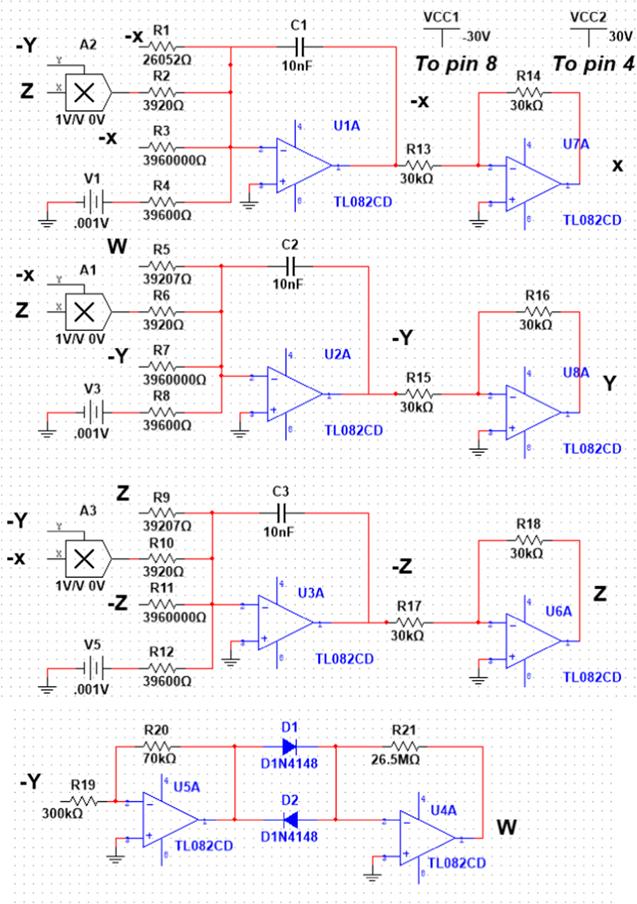
Figure 13. Schematic view of system (8), using MultiSIM 14.1. |
4.2. Analog simulation
Table 3. The values of resistors and voltages for capacitors ${C}_{1}={C}_{2}={C}_{3}=10\,{\rm{nF}}$ for different values of $\alpha .$ |
| $\alpha $ | Voltage (${\rm{V}}$) | Resistor ($k{\rm{\Omega }}$) | $\alpha $ | Voltage (${\rm{V}}$) | Resistor ($k{\rm{\Omega }}$) | ||||
|---|---|---|---|---|---|---|---|---|---|
| 1.00 | ${V}_{1}$ | — | ${R}_{1}$ | 20 | 0.92 | ${V}_{1}$ | 0.009 | ${R}_{1}$ | 24.29 |
| ${R}_{2}$ | 3 | ${R}_{2}$ | 3.63 | ||||||
| ${R}_{3}$ | 30 | ${R}_{3}$ | 440 | ||||||
| ${V}_{2}$ | — | ${R}_{4}$ | 3 | ${V}_{2}$ | 0.009 | ${R}_{4}$ | 39.60 | ||
| ${R}_{5}$ | 30 | ${R}_{5}$ | 36.33 | ||||||
| ${R}_{6}$ | 3 | ${R}_{6}$ | 3.63 | ||||||
| ${V}_{3}$ | — | ${R}_{7}$ | — | ${V}_{3}$ | 0.009 | ${R}_{7}$ | 440 | ||
| ${R}_{8}$ | — | ${R}_{8}$ | 39.60 | ||||||
| ${R}_{9}$ | — | ${R}_{9}$ | 36.33 | ||||||
| ${R}_{10}$ | — | ${R}_{10}$ | 3.63 | ||||||
| ${R}_{11}$ | — | ${R}_{11}$ | 440 | ||||||
| ${R}_{12}$ | — | ${R}_{12}$ | 39.60 | ||||||
| 0.99 | ${V}_{1}$ | 0.001 | ${R}_{1}$ | 26.05 | 0.90 | ${V}_{1}$ | 0.011 | ${R}_{1}$ | 23.76 |
| ${R}_{2}$ | 3.92 | ${R}_{2}$ | 35.64 | ||||||
| ${R}_{3}$ | 3960 | ${R}_{3}$ | 356.75 | ||||||
| ${V}_{2}$ | 0.001 | ${R}_{4}$ | 39.60 | ${V}_{2}$ | 0.011 | ${R}_{4}$ | 39.60 | ||
| ${R}_{5}$ | 39.20 | ${R}_{5}$ | 35.64 | ||||||
| ${R}_{6}$ | 3.920 | ${R}_{6}$ | 3.564 | ||||||
| ${V}_{3}$ | 0.001 | ${R}_{7}$ | 3960 | ${V}_{3}$ | 0.011 | ${R}_{7}$ | 356.75 | ||
| ${R}_{8}$ | 39.60 | ${R}_{8}$ | 39.60 | ||||||
| ${R}_{9}$ | 39.20 | ${R}_{9}$ | 35.64 | ||||||
| ${R}_{10}$ | 3.92 | ${R}_{10}$ | 3.564 | ||||||
| ${R}_{11}$ | 3960 | ${R}_{11}$ | 356.75 | ||||||
| ${R}_{12}$ | 39.60 | ${R}_{12}$ | 39.60 | ||||||
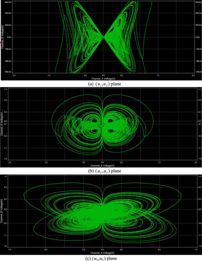
Figure 14. Analogous phase plots of system (8) where $\alpha =1.00.$ |
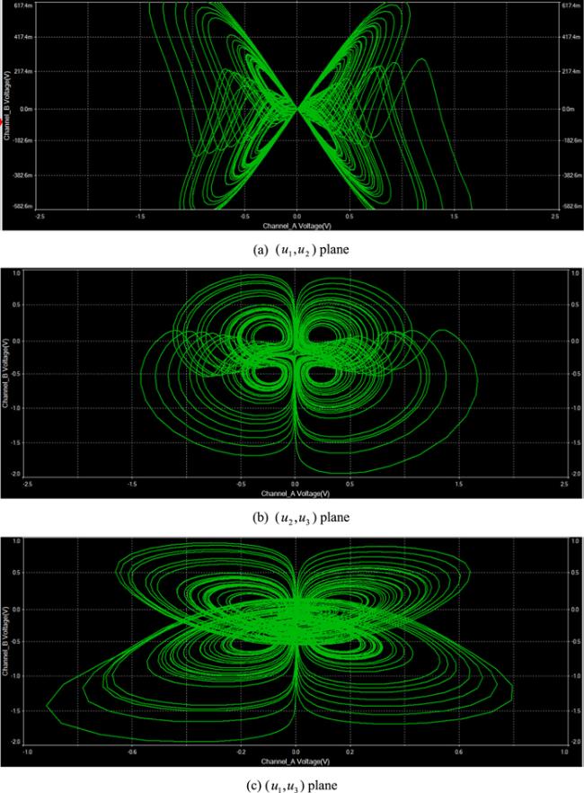
Figure 15. Analogous phase plots of system (8) where $\alpha =0.99.$ |
4.3. Cryptographic simulation
Table 4. ${\rm P}$-value test results (NIST-800-22) for chaotic series ${u}_{1}\left(t\right),$ at different values of $\alpha .$ |
| S. No | Test Name | $\alpha $ = 1 | $\alpha $ = 0.99 | $\alpha $ = 0.92 | Results |
|---|---|---|---|---|---|
| 1 | Mono bitFrequency Test | 0.665 006 | 0.484 806 | 0.317 884 | Successful |
| 2 | Block Frequency Test | 0.678 612 | 0.985 867 | 0.518 35 | Successful |
| 3 | Runs Test | 0.707 856 | 0.193 446 | 0.360 131 | Successful |
| 4 | Longest Runs Ones 10 000 | 0.235 903 | 0.556 629 | 0.063 0856 | Successful |
| 5 | Binary Matrix Rank Test | 0.443 084 | 0.298 222 | 0.045 5016 | Successful |
| 6 | Spectral Test | 0.474 456 | 1. | 0.458 246 | Successful |
| 7 | Non-Overlapping Template Matching | 0.529 55 | 0.840 569 | 0.488 286 | Successful |
| 8 | Overlaping Template Matching | 0.544 82 | 0.981 736 | 0.375 187 | Successful |
| 9 | Maurers universal Statistic Test | 0.463 56 | 0.183 854 | 0.385 959 | Successful |
| 10 | Linear Complexity Test | 0.701 088 | 0.515 697 | 0.503 53 | Successful |
| 11 | Serial Test | {0.259 896,0.713 345} | {0.326 326,0.718 48} | {0.760 873,0.839 907} | Successful |
| 12 | Approximate Entropy Test | 0.344 719 | 0.223 394 | 0.141 817 | Successful |
| 13 | Cumulative Sums Test | 0.638 251 | 0.825 325 | 0.593 75 | Successful |
| 14 | Random Excursions Test | 0.296 283 | 0.194 65 | 0.123 997 | Successful |
| 15 | Random Excursions Variant Test | 1 | 0.245 779 | 0.863 832 | Successful |
| 16 | Cumulative Sums Test Reverse | 0.976 076 | 0.822 779 | 0.593 75 | Successful |
Table 5. ${\rm P}$-value test results (NIST-800-22) for chaotic series ${u}_{2}\left(t\right),$ at different values of $\alpha .$ |
| S. No | Test Name | $\alpha $ = 1 | $\alpha $ = 0.99 | $\alpha $ = 0.92 | Results |
|---|---|---|---|---|---|
| 1 | Mono bitFrequency Test | 0.716 059 | 0.953 96 | 0.367 766 | Successful |
| 2 | Block Frequency Test | 0.638 647 | 0.474 88 | 0.617 961 | Successful |
| 3 | Runs Test | 0.004 748 35 | 0.567 602 | 0.784 317 | Successful |
| 4 | Longest Runs Ones 10 000 | 0.692 827 | 0.933 756 | 0.377 388 | Successful |
| 5 | Binary Matrix Rank Test | 0.332 02 | 0.180 156 | 0.903 766 | Successful |
| 6 | Spectral Test | 0.289 315 | 0.524 923 | 0.542 336 | Successful |
| 7 | Non-Overlapping Template Matching | 0.873 754 | 0.329 533 | 0.137 408 | Successful |
| 8 | Overlaping Template Matching | 0.366 99 | 0.422 48 | 0.279 795 | Successful |
| 9 | Maurers universal Statistic Test | 0.336 621 | 0.535 156 | 0.844 607 | Successful |
| 10 | Linear Complexity Test | 0.229 947 | 0.969 042 | 0.224 795 | Successful |
| 11 | Serial Test | {0.235 703,0.593 431} | {0.574 309,0.443 98} | {0.864 631,0.918 161} | Successful |
| 12 | Approximate Entropy Test | 0.023 8884 | 0.586 246 | 0.249 462 | Successful |
| 13 | Cumulative Sums Test | 0.983 936 | 0.840 404 | 0.627 666 | Successful |
| 14 | Random Excursions Test | 0.769 331 | 0.804 348 | 0.316 433 | Successful |
| 15 | Random Excursions Variant Test | 0.947 793 | 0.388 667 | 0.331 918 | Successful |
| 16 | Cumulative Sums Test Reverse | 0.727 184 | 0.788 972 | 0.263 668 | Successful |
Table 6. ${\rm P}$-value test results (NIST-800-22) for chaotic series ${u}_{3}\left(t\right),$ at different values of $\alpha .$ |
| S. No | Test Name | $\alpha $ = 1 | $\alpha $ = 0.99 | $\alpha $ = 0.92 | Results |
|---|---|---|---|---|---|
| 1 | Mono bitFrequency Test | 0.981 575 | 0.623 605 | 0.724 701 | Successful |
| 2 | Block Frequency Test | 0.702 138 | 0.786 538 | 0.330 245 | Successful |
| 3 | Runs Test | 0.145 69 | 0.463 838 | 0.724 432 | Successful |
| 4 | Longest Runs Ones 10 000 | 0.746 165 | 0.415 693 | 0.423 45 | Successful |
| 5 | Binary Matrix Rank Test | 0.685 773 | 0.574 195 | 0.570 329 | Successful |
| 6 | Spectral Test | 0.194 273 | 0.633 482 | 0.474 456 | Successful |
| 7 | Non-Overlapping Template Matching | 0.834 296 | 0.498 41 | 0.512 831 | Successful |
| 8 | Overlaping Template Matching | 0.219 927 | 0.664 717 | 0.230 988 | Successful |
| 9 | Maurers universal Statistic Test | 0.235 758 | 0.139 78 | 0.688 589 | Successful |
| 10 | Linear Complexity Test | 0.709 004 | 0.523 366 | 0.803 015 | Successful |
| 11 | Serial Test | {0.412 075,0.209 017} | {0.197 128,0.442 195} | {0.437 12,0.534 607} | Successful |
| 12 | Approximate Entropy Test | 0.734 978 | 0.135 837 | 0.845 66 | Successful |
| 13 | Cumulative Sums Test | 0.845 347 | 0.770 349 | 0.791 612 | Successful |
| 14 | Random Excursions Test | 0.654 05 | 0.281 157 | 0.428 759 | Successful |
| 15 | Random Excursions Variant Test | 0.262 747 | 0.326 878 | 0.391 404 | Successful |
| 16 | Cumulative Sums Test Reverse | 0.825 325 | 0.360 73 | 0.635 598 | Successful |
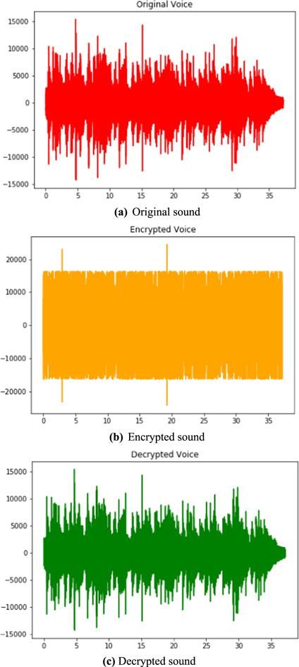
Figure 16. Sound data. |

Figure 17. Magnitude spectrum of sound. |
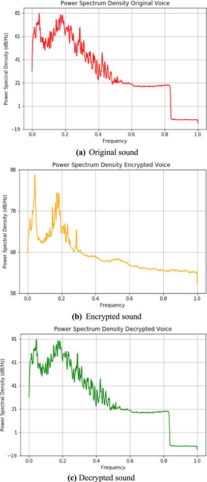
Figure 18. Power spectrum density of sound data. |
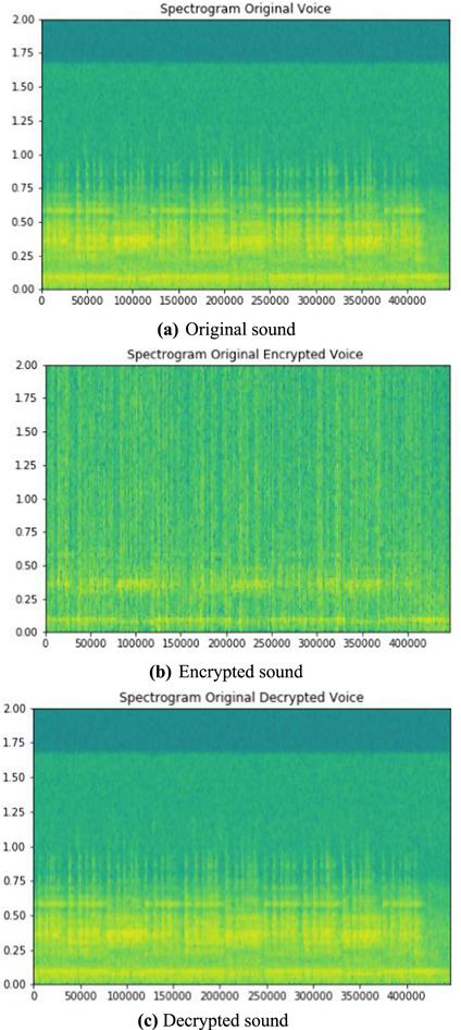
Figure 19. Spectrogram of sound data. |
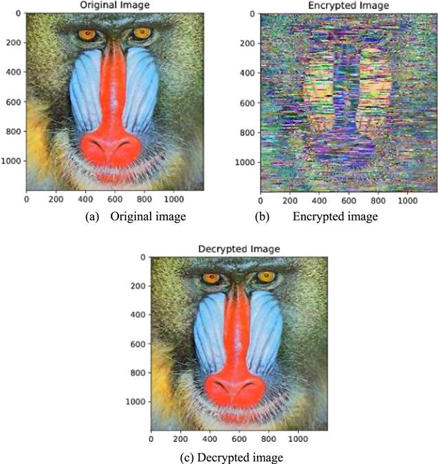
Figure 20. Cryptographic test on image 1 (Mandrill). |
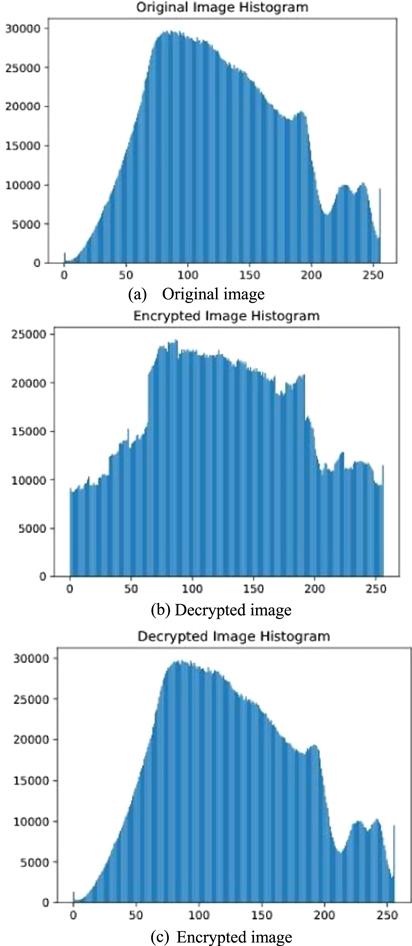
Figure 21. Histogram of cryptographic test on image 1. |
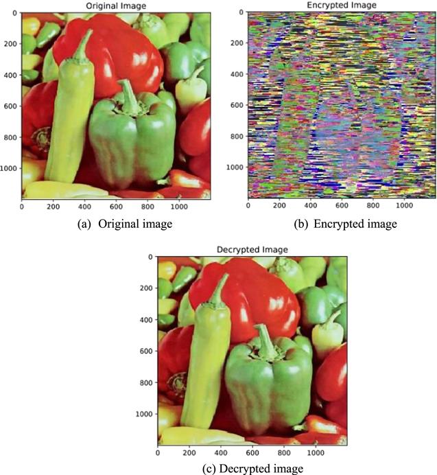
Figure 22. Cryptographic test on image 2 (Peppers). |
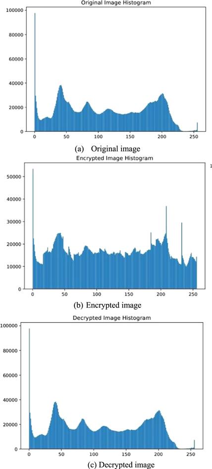
Figure 23. Histogram of cryptographic test on image 2. |
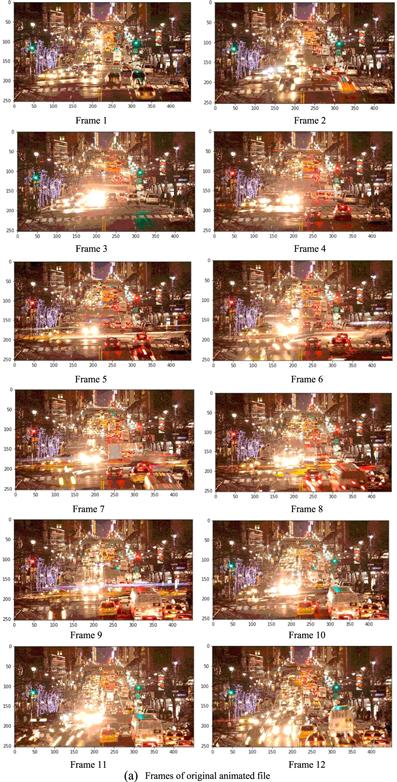
Figure 24. Frames from an animated (.gif) file original, encrypted, and decrypted, together with the corresponding histograms. |
4.4. Security analysis
4.4.1. Histogram analysis
4.4.2. Key sensitivity analysis
| NPCR:The number of pixel change rate (NPCR) can be expressed as follows: $\begin{eqnarray*}\begin{array}{l}{\rm{N}}{\rm{P}}{\rm{C}}{\rm{R}}=\displaystyle \sum _{i=1}^{M}\displaystyle \sum _{j=1}^{N}\left[\displaystyle \frac{D\left(i,j\right)}{M\times N}\right]\times 100 \% ,\,{\rm{with}}\\ D\left(i,j\right)=\left\{\begin{array}{cc}0 & {C}_{1}\left(i,j\right)={C}_{2}\left(i,j\right)\\ 1 & otherwise\end{array}\right..\end{array}\end{eqnarray*}$ Here, ${C}_{1}\left(i,j\right)$ and ${C}_{2}\left(i,j\right)$ denote the pixel values of the two encrypted images, where the originals possess only one pixel difference, respectively, at the ith pixel row,and the jth pixel column. | |
| UACI: The unified average changing intensity (UACI) can be written as follows: |
4.4.2.1. Information entropy analysis
| Entropy indicates the randomness of a system, and can be calculated as follows: |
Table 7. Numerical values of Parameters for security analysis. |
| Entropy | ||||
|---|---|---|---|---|
| Test images | NPCR (%) | UAIC (%) | Plain Image | Encrypted Image |
| Mandrill | 98.958 079 | 21.426 310 | 5.333 076 | 5.777 796 |
| Peppers | 99.104 309 | 24.509 208 | 4.342 038 | 5.742 104 |
5. Conclusion
| • | The multi-wing system possesses multi-stability equilibrium points at distinct values of $\alpha .$ |
| • | The physical parameters of the model can be simulated by means of circuit design. |
| • | Many keys can be generated to form sheltered systems for data communication. |
| • | The proposed mechanism has the capacity to track files in different formats. |
| • | This system is also suitable for other chaos-based applications. |