


1. Introduction
Cell size control is an important topic in bacterial physiology [1]. Bacterial volume has a wide range, spanning over seven orders of magnitude, from 0.01 μm3 [2] to 2 × 105 μm3 [3], and bacteria have various cell shapes, such as coccus (spherical), bacillus (rod-shaped), and spiral (twisted) [4]. Despite this diversity, individual organisms have a preferred size with a very narrow distribution, like E.coli with a coefficient of variation, CV = s.d./mean, of birth cell size distribution only being 10% [5, 6]. The phenomenon is called cell size homeostasis. Individual cell size homeostasis was also found in animals [7, 8] and fission yeast [9]. How to control cell size to a stable and narrow distribution, and the molecular mechanism of cell size control count for much in cell biology [10].
The cell volume can be measured at the population or single-cell level. In 1958, Schaechter, Maalφe, and Kjeldgaard found a relationship between growth rate and cell volume named Schaechter–Maalφe–Kjeldgaard (SMK) growth law [11, 12]. The growth law was also called as nutritional growth law, confirmed by Sattar Taheri-Araghi et al [13] at the single-cell level. The nutritional growth law indicates that the average cell birth volume increases exponentially with the growth rate in different given growth condition. That is:
$\begin{eqnarray}V={{\rm{e}}}^{\mu Y+X},\end{eqnarray}$
where V is the average birth volume, μ the growth rate, Y and X being growth-rate-independent constants. The SMK growth law was interpreted as a result of cells adapting to the external condition [14–16]. Larger cells with faster growth rates possess more DNA and more cytoplasm [12]. Another important result of the SMK experiment is that cells growing at different growth rates have different chemical components. The logarithms of cell constituents (protein per cell, DNA per cell, and RNA per cell) are proportional to the growth rate. It should be noted that the growth rate μ in the SMK growth law is the population exponential growth rate, and it is different from the elongation rate at single-cell level. The population growth rate is the ensemble average of the elongation rate. The SMK growth does not mean that cells with faster elongation rate have a lager volume in the same culture condition. Cell homeostasis is a conception in same culture condition. So the SMK growth law does not contradict size homeostasis. How cell size and cell components are determined by cell growth rate is one of the major topics to be investigated in the field of bacterial physiology.Cell size control has to accommodate with cell cycle, which determines when to initiate DNA replication, when to complete DNA replication, and when to divide [17, 18]. In 1968, Donachie [19] put forward a vital model, indicating that:
$\begin{eqnarray}V(\tau )={V}_{0}{2}^{(C+D)/\tau },\end{eqnarray}$
where V(τ) is the average cell size at the birth time or called constant initiation size, V0 the average cell size per origin (Origin means the origin of replication, a specific DNA sequence in a genome at which replication starts.) at the time of DNA replication initiation, C the duration of replication, D the time to segregate the chromosomes and divide, and τ average cell doubling time. C + D is about 60 min in experiments between replication initiation and cell division called cell cycle time. In our work, the cell cycle time is defined as chromosome replication cycle time, which is from the initiation of DNA replication to the sister chromosomes segregation. It is different from doubling time or generation time, which is the time between two consecutive divisions. Donachie’s work was based on two cornerstone assumptions [20, 21]: (i) the chromosome replication time (C period) is a constant during the steady growth in whatever growth condition; (ii) the time between replication initiation and cell division (C + D period) is a constant. In 2015, Sattar Taheri-Araghi et al [13] examined Donchie’s model at the single-cell level. Under extensive growth inhibition conditions, cell size at replication initiation per origin is also invariant [22].There are three theoretical models to interpret how cells control their cell size: adder [13, 23], sizer [24], and timer [25]. Adder regulation means that cells add a fixed increment between two division events, sizer regulation meaning that cell division or chromosome replication begins when cell size reaches a critical value, and timer means the time across the cell cycle is a constant. Assuming the correlation between mother and daughter birth sizes is α, then the daughter cell size can be expressed by the following formula [17, 18]:
$\begin{eqnarray}{V}^{+1}=\alpha {V}^{0}+(1-\alpha ){V}^{m}+\xi ,\end{eqnarray}$
where V+1 is the daughter birth size, V0 the mother birth size, Vm the population average birth size, and ξ Gaussian white noise. If cells grow exponentially, then timer regulation results in α = 1, adder regulation resulting in α = 1/2, and sizer regulation resulting in α = 0. So the correlations between birth size and division size can be used to distinguish three models. With single-cell technology development, it is easy to get the correlations between birth size and division size, as well as the correlations between birth size and inter-division time. Recently researches have demonstrated that bacteria achieve cell size homeostasis through adder model [13, 23, 26–29].The adder property is of core importance in the field of bacterial physiology [30]. There are many phenomenological models [28, 31–33] explaining the adder property, the correlation between birth volume and division volume, and the correlation between inter-division time and birth volume. Recent studies [34, 35] have demonstrated the adder property arises in not only the birth-division process but also the DNA replication cycle. These works showed that the adder property requires protein accumulation to a threshold to begin DNA replication or cell division and balanced biosynthesis during cell elongation. In the following sections, we will affirm the double-adder model in silicon.
2. Model
We established a model like Precursor–Transporter–Ribosome cell model in the works [30, 36, 37]. We considered the cell model containing four sectors: precursors, metabolic proteins, ribosomes, and housekeeping proteins, as displayed in figure 1. Precursors molecules consist of 20 kinds of amino acids. Metabolic proteins include transporter transporting the external food into the cell and proteins converting food into amino acids. Ribosomes are self-catalytic proteins, making amino acids into various proteins. Housekeeping proteins are proteins that maintain the physiological stability of cells. The proportion of housekeeping proteins is considered to be a constant.
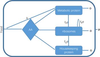
Figure 1. A coarse-grained model of the cell. Extracellular food is transported into the cell and is decomposed into amino acids (AA) by metabolic proteins. Amino acids are assembled into various proteins by ribosomes and are allocated to metabolic proteins, ribosomes, and housekeeping proteins reasonably to get a maximal growth rate. → φ means the degradation of proteins. μ is the growth rate. |
The model is described by the following set of differential equations:
$\begin{eqnarray}\displaystyle \frac{{\rm{d}}A}{{\rm{d}}t}={kT}-\sigma \displaystyle \frac{{RA}}{V},\end{eqnarray}$
$\begin{eqnarray}\displaystyle \frac{{\rm{d}}T}{{\rm{d}}t}=\displaystyle \frac{{f}_{T}\sigma }{{n}_{T}}\displaystyle \frac{{RA}}{V}-{d}_{T}T,\end{eqnarray}$
$\begin{eqnarray}\displaystyle \frac{{\rm{d}}R}{{\rm{d}}t}=\displaystyle \frac{{f}_{R}\sigma }{{n}_{R}}\displaystyle \frac{{RA}}{V}-{d}_{R}R,\end{eqnarray}$
$\begin{eqnarray}\displaystyle \frac{{\rm{d}}Q}{{\rm{d}}t}=\displaystyle \frac{{f}_{Q}\sigma }{{n}_{Q}}\displaystyle \frac{{RA}}{V}-{d}_{Q}Q,\end{eqnarray}$
where A represents the number of precursors molecules or amino acids, T the number of metabolic proteins including transporter proteins transporting food into the cell and proteins converting food into precursor, R the number of ribosomes and Q the number of housekeeping proteins. V is the cell volume: $\begin{eqnarray}V={gm}=g({m}_{A}A+{n}_{T}{m}_{A}T+{n}_{R}{m}_{A}R+{n}_{Q}{m}_{A}Q),\end{eqnarray}$
where g means unit mass protein occupying volume, it is reasonable to assume that g is a constant because the variation of cell dry-mass density is very small [38]. mA is the average mass of a single amino acid, and nT, nR and nQ are the average numbers of amino acids consisting of metabolic proteins, ribosomes, and housekeeping proteins, respectively. k represents the efficiency of metabolism, which is a function of external food concentration and food quality. Σ is the ribosomal catalytic efficiency, the rate of amino acid consumption for a single ribosome per unit amino acids concentration. dT, dR and dQ are the degradation rate of metabolic proteins, ribosomes, and housekeeping proteins, respectively. fT, fR and fQ represent the fractions of ribosomes engaged in making metabolic proteins, ribosomes, and housekeeping proteins, respectively. Their sum satisfies: $\begin{eqnarray}{f}_{T}+{f}_{R}+{f}_{Q}=1,\end{eqnarray}$
where fQ is a constant.When cell grows exponentially with a growth rate μ, it is easy to get a quadratic polynomial expression of growth rate:appendix . Its solution proves Monod growth law [39]:appendix .
$\begin{eqnarray}{a}_{2}{\mu }^{2}+{a}_{1}\mu +{a}_{0}=0,\end{eqnarray}$
where the coefficients a0, a1 and a2 depend on the food concentration, food quality, physical constants, and ribosomal catalytic efficiency, defined in the $\begin{eqnarray}\mu =\displaystyle \frac{1}{2}(1-{f}_{Q})\displaystyle \frac{\rho \nu }{\rho +\nu },\end{eqnarray}$
where ρ, ν are defined in Now we introduce trigger proteins. I and D are the molecules that control DNA replication initiation and cell division respectively. Their dynamics are determined by4 )–(13 ) show that the number of chemical population is proportional to cell size V, so that the production rate of chemical population is proportional to cell size V. We referred to our model as an ATRQID system.
$\begin{eqnarray}\displaystyle \frac{{\rm{d}}I}{{\rm{d}}t}={K}_{I}\displaystyle \frac{{RA}}{V},\end{eqnarray}$
$\begin{eqnarray}\displaystyle \frac{{\rm{d}}D}{{\rm{d}}t}={K}_{D}\displaystyle \frac{{RA}}{V},\end{eqnarray}$
where KI and KD are rate constants. When the number of I or D reaches a threshold respectively, chromosome replication or cell division begins. Because the number of DnaA and the number of FtsZ per cell are very limited [40, 41], the mass of cell size regulators is negligible to the whole cell. As the equations (Our model has many limitations. Our model does not include the complete genetic central law. We did not consider the effect of gene copy number on transcription rate and translation rate [42]. The sources of gene expression noise are very extensive and complex. Our model is too simple to consider so many influencing factors.
3. Deterministic results
As the parameters of the dynamical system ATRQID sector are specified and chemical populations are given initial values, the system will go on forever. The deterministic dynamic of the ATRQID system is discussed in this section, and the stochastic dynamic will be discussed in the following sections.
Thus, as the number of DNA replication protein I per origin reaches the threshold Ic, DNA replication begins, and I per origin degrades to Ir (Ir < Ic) per origin. As the number of division protein, D reaches the threshold Dc, the cell divides without any delay, and the population of A, T, R, Q, and I are halved, while the number of division protein is set to Dr(Dr < Dc). The populations’ dynamics follow the equations (4 )–(13 ), and the process is repeated and repeated. The deterministic simulation results are shown in figure 2. Most parameters of the ATRQID sector are chosen from realistic experiment values and can reproduce known experimental data of E.coli, shown in table 1. Adder property was found from prokaryotes to animal cells. Different doubling times and birth size cells do not influence the adder property. To show sharp contrasts, we fixed the rate parameters except sections 4.4 and 4.5 .
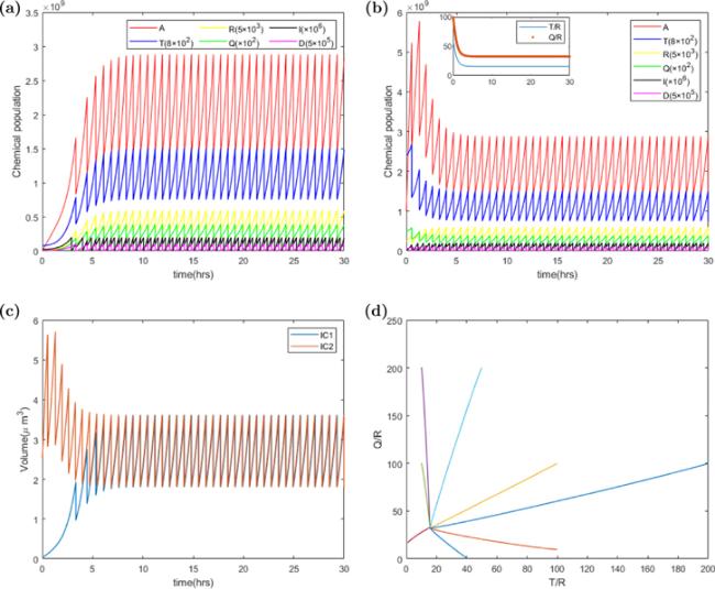
Figure 2. The deterministic trajectories of chemical populations, P, T, R, Q, I, D and volume V versus time t. Parameters of the ATRQID system are k = 3000 h−1, Σ = 3 ∗ 10−5 μm3 h−1, KD = 4 ∗ 10−12 h−1, KI = 6 ∗ 10−12 h−1, dR = dQ = dT = 0.1 h−1, Dc = 200, Ic = 200, Dr = 0, Ir = 0, and the other parameters of the model are shown in the table 1. The population values in (a) and (b) have been adjusted to make all of populations shown on the same figure by some multiplier factors. (a) The trajectory of populations versus time in a cell with the initial condition IC1: A(0) = 103, T(0) = 105, R(0) = 103, Q(0) = 104, I(0) = 20, D(0) = 10. The populations’ dynamics evolve to a steady state, and the chemical populations in the daughter cell at the birth are Ab = 1.28 ∗ 109, Tb = 8.39 ∗ 105, Rb = 5.26 ∗ 104, Qb = 1.71 ∗ 106, Ib = 88, Db = 0. The doubling time is 0.7235 h. (b) The trajectory of populations versus time in a cell with the initial condition IC2: A(0) = 109, T(0) = 3∗106, R(0) = 5∗104, Q(0) = 5∗106, I(0) = 10, D(0) = 100. The population dynamics reach a same steady state as IC1. (c) The plot of cell size versus time on the two initial conditions IC1 and IC2. (d) The 2D space of Q/R and T/R shows that the trajectories converge to the same attractor independent of initial conditions. |
Table 1. The dynamics parameters and biological constants in the ATRQID system. |
| Constants/Parameters | Symbol | Value | Reference |
|---|---|---|---|
| Protein density | g | 0.25 g cm−3 | [76] |
| Molecular weight per ribosome R | nR | 7336aa | [75] |
| Molecular weight per metabolic protein T on average | nT | 325aa | [70] |
| Molecular weight per housekeeping protein P on average | nQ | 325aa | [70] |
| Protein degradation rate respectively | dR, dT, dQ | Given | [71, 72] |
| The efficiency of metabolic enzymes T | k | Given | |
| Ribosomal catalytic efficiency | Σ | Given | |
| The fractions of ribosomes engaged in making ribosomes R | fR | Optimized by growth rate | Equation ( |
| The fractions of ribosomes engaged in making metabolic protein T | fT | Optimized by growth rate | Equation ( |
| The fractions of ribosomes engaged in making housekeeping protein T | fQ | 0.45 | [73] |
| DNA replication initiation protein per origin threshold | Ic | Given | |
| Cell division initiation protein threshold | Dc | Given | |
| The average mass of amino acids | mA | 3000Da | [74] |
| DNA replication initiation protein synthesis rate constant | KI | Given | |
| Cell division initiation protein synthesis rate constant | KD | Given |
As shown in figures 2(a) and (b), after a short transitional state depending on the initial condition, the chemical populations gathered to a steady state independent of the initial condition. The population number and cell volume got to maximum when the number of cell division proteins got to the threshold, and chemical population and cell size were halved. The dynamics system was an attractor making the populations grow at the same rate, i.e. the numbers of various proteins doubling times are the same, as displayed in figure 2(d).
4. Stochastic numerical results
As displayed above, we made a deterministic simulation of the dynamics trajectories of the ATRQDI cell. Now we show the stochastic version as posed in figure 3. The differences between the deterministic version and the stochastic version are: (i) the population’s number is an integer and updated by Gillespie algorithm [43, 44], (ii) the DNA replication protein threshold is a random variable following Poisson distribution with mean Ic. When I reaches its target, the chromosome replication begins, the number of origins doubles, then I is broken down to Ir(Ir < Ic/2), (iii) the division protein threshold is a random variable following Poisson distribution with mean Dc. When the division protein D reaches the threshold, the cell begins to split into two daughter cells, after that D is degraded to Dr(Dr < Dc/2). The cell is divided into two approximate same daughter cells satisfying normal distribution.
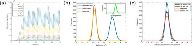
Figure 3. The stochastic trajectories and the scale-free property of cell size. (a) The stochastic trajectories of chemical populations, P, T, R, Q, I, D and volume V versus time t. Parameters of the dynamics systems are k = 3000 h−1, Σ = 3 ∗ 10−5 μm3 h−1, KD = 4 ∗ 10−12 h−1, KI = 6 ∗ 10−12 h−1, dR = dQ = dT = 0.1 h−1, Dc = 200, Ic = 200, Dr = 0, Ir = 0, and the other parameters of the model are shown in the table 1. The population values in figure 3(a) have been adjusted to make all of populations shown on the same figure by some multiplier factors. (b) The frequency distribution of cell division size, birth size, added size, and inter-division time in the steady state. The average division cell size ⟨Vd⟩ is 3.279 μm3, average birth cell size ⟨Vb⟩ = 1.642 μm3, average added cell size ⟨Δ⟩ = 1.637 μm3, average division time ⟨τ⟩ = 0.723 h. (c) The frequency distribution of cellular variables is re-scaled by their respective means. The curves denoted by cell division size, cell birth size, added size and doubling time stand for Vd/⟨Vd⟩, Vb/⟨Vb⟩, Δ/⟨Δ⟩ and τ/⟨τ⟩. The coefficient of variation of those cellular variables are 0.071, 0.093, 0.113, 0.094. |
We found that after several cycles of growth, division, and birth, the system got to a steady state, where all of the chemicals have balanced biosynthesis. Different from the deterministic version, the daughter cell in the stochastic simulation is not the same due to stochastic initiation and division. The parameters in figure 3(a) are the same as those in figure 2(a).
A surprising phenomenon is that the distribution of cell birth size is only the function of the mean cell size both in the intra-species [13] and inter-species [45] level. This phenomenon implies that most cells share the same division mechanism, so the distribution of cell birth size can be rescaled by the average birth size. The growth rate cannot be rescaled by the mean growth rate [46]. Because the growth rate influences the age distribution of cell, so the cell size distribution of population snapshot data and the cell size distribution of cell lineage data are growth rate-dependent. The article [13] displays that the relationship between the variation of cell division size, birth size, added size, and inter-division time is expressed by:
$\begin{eqnarray}\sqrt{3}{\rm{CV}}({V}_{d})\approx \sqrt{3}{\rm{CV}}({V}_{b})\approx 1/\sqrt{\mathrm{ln}2}{\rm{CV}}(\tau )\approx {\rm{CV}}({\rm{\Delta }}),\end{eqnarray}$
where Vd is the cell division cell, Vb cell birth size, Δ = Vd − Vb added size or the cell size increased between division time, and τ doubling time. We performed 20 000 stochastic division simulations for our model with the same condition in figure 2(a); then, we tracked the cellular variables for all the cells in one trajectory. We observed the averages of the steady state as shown in figures 3(b) and (c): the average division cell size ⟨Vd⟩ = 3.279 μm3, average birth cell size ⟨Vb⟩ = 1.642 μm3, average added cell size ⟨Δ⟩ = 1.637 μm3, average division time ⟨τ⟩ = 0.723 h. The coefficient of variation of those cellular variables are 0.071, 0.093, 0.113, 0.094 respectively, while the work [13] showed that CV of four quantities are 0.12, 0.139, 0.156, and 0.2, respectively. Our noise results are smaller than work [13]. CV of added size is biggest, and CV of division size, birth size, and doubling time are approximately the same. The results are similar with work [13]. So our results are not all consistent with the article [13]. It is maybe because we did not consider the noise of growth rate [47].What is the distribution of cell size at birth is a very controversial issue. As shown in the figure 4(a), we used three distributions to fit our data. Like most experimental data, our data does not distinguish these three distributions very well. Cell size distribution of lineage data is a quirky curve [48]. Fortunately, as displayed in figure 4(b) our simulation results captured the three most important characteristics of this distribution: when it is smaller than the most probable size of the cell, the number of cells rises rapidly; after that, the number of cells begins to decrease slowly; when the cell size reaches a certain value, the number of cells begins to decrease rapidly.

Figure 4. The cell birth size distribution versus cell size distribution of lineage data. (a) In the same lineage, the distribution of tens of thousands of consecutive cells at birth. Three distributions are used to fit this distribution, namely: Gaussian distribution, gamma distribution, and lognormal distribution. (b) In the same lineage, the cell size distribution of cell lineage data for dozens of consecutive generations. |
When we analyze bacterial physiology, there are two pictures: one is paying close attention to the cell division, and the other is focusing on DNA replication. We drew a simple diagram figure 5 to show the differences between the two pictures. The relationship between cell division and cell cycle is vital and studied extensively.
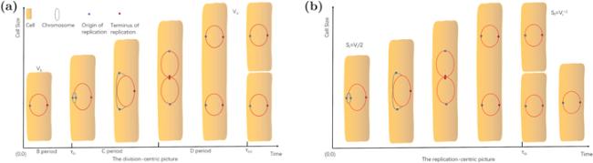
Figure 5. The division-centric picture and the replication-centric picture of the cell cycle. (a) In the division-centric picture, the cell cycle is separated into three periods. The first period is from cell birth to initiation of DNA replication, named B period. The second period is the time interval DNA replication occupies, called C period. The last one is from the completion of the chromosome of replication to cell division, named D period. DNA replication begins at the origin when the cell size reaches a critical volume Vi and ends at the terminus. (b) The replication-centric picture is defined as two consecutive chromosome replication initiations. It is worth noting that (b) is only tenable at a slow growth rate. When doubling time is shorter than C + D, there will be more than one round replication in the cell. All the biological variables are defined in table 2. |
When we research the question about cell size, using the division-centric picture is natural. In the picture, the period is from cell birth to cell division. The Pearson correlations between cell birth size, cell division size, doubling time, and added size are used by investigators to estimate which size regulation mechanism is adopted by cells. Another two important variables are chromosome replication initiation time and completion time. From cell birth to replication initiation is named B period, the time to replicate the chromosome C period and the time replication completion to cell division D period. In general C period and D period are thought independent, and C + D is a constant [19]. But recent researches dedicates that C + D is growth-rate-dependent [34, 49].
What is different from the division-centric picture is that the replication-centric picture is from replication initiation to the subsequent replication initiation. Recently more and more researchers began to realize the importance of cell size regulation in the replication-centric picture [18]. Amir [18] believes that there is no specific cell size regulatory mechanism, and cell size homeostasis originates from the control of chromosome replication.
The adder property between cell division is one general phenomenon that is still required to explain. The adder property also emerges between consecutive replication initiation [34, 35]. In the following sections, our work will reveal the adder property is only based on two basic assumptions: (i) a fixed number target of cell division protein to trigger division, a threshold of DNA replication protein to touch off replication, and then proteins are degraded or deactivated. (ii) All the chemical populations are produced by a rate proportional to the cell size, i.e. balanced biosynthesis. So we got the conclusion that not only cell division but also DNA replication was important to cell size regulation, but cell size homeostasis was irrelevant to chromosome replication initiation.
4.1. The adder property of division-centric picture
We collected 20 000 cells in one stochastic trajectory, and then we gathered the biological quantities, including the chemical population numbers, cell size, origin number at cell division time, and chromosome replication initiation time. After that, we calculated the mean chemical population numbers, mean cell size, the distribution of cell size at different important time nodes. By using 20 000 successive cells in one trajectory, we computed the Pearson correlation coefficient between added volume Δ, division volume Vd, doubling time τ, cell size at replication initiation, and birth cell size Vb, displayed in figure 6. We found that the ATRQID system displayed the adder property, the mean added volume Δ independent of birth cell size. We found a significant result that the birth size was positive correlative with cell size at DNA replication initiation. This conclusion does not support the constant initiation mass assumption [19, 34, 37, 50] by Donachie in 1968. So the chromosome replication initiation is not controlled by cell mass but rather the number of replication initiation protein. Our result is consistent with work [34].
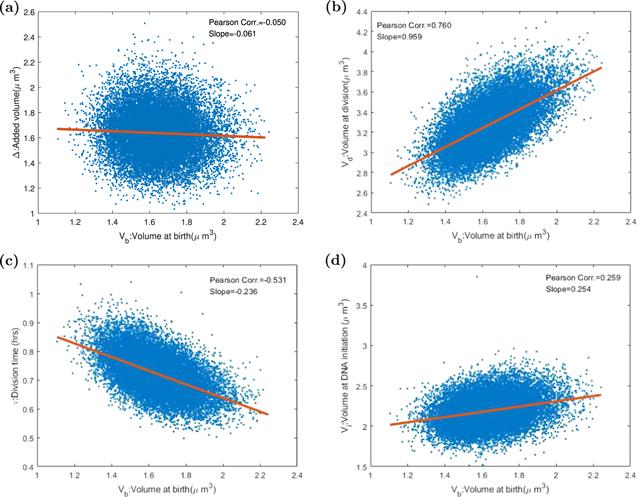
Figure 6. The Pearson correlation coefficients and slopes between various variables in the division-centric picture. Each point stands for one cell in 20 000 consecutive divisions after the system gets into the steady state. The red line is the linear fitting curve. (a) The X-axis refers to the cell birth volume, and the Y-axis refers to the increased volume during the division cycle. In the ideal adder model, the correlation coefficient of Vb and Δ should be 0. Our result is −0.050, so that add property is proved in our model. (b) The correlation coefficient of Vb, volume at birth time, and Vd, volume at division time, is 0.760. The slope of the fitting curve is about 1. (c) The doubling time τ is negatively correlated with birth size. In the ideal adder model, the correlation coefficient should be −0.5, compared with our model −0.531. (d) The replication initiation size Vi is positively correlated with Vb with the correlation coefficient being 0.259. If Donchie’s hypothesis is correct, the value should be 0. |
4.2. The adder property of replication-centric picture
As the same as the division-centric picture, using 20 000 successive cells in one trajectory, we computed biological variables in the replication-centric picture. As defined in table 2 and shown in figure 5, volume per origin at replication initiation is Si = Vi/2, volume at final replication initiation Sf being same as the volume ${V}_{i}^{+1}$ at next round of replication initiation, added volume between replication cycle Δif = Sf − Si. It is worth reminding that for the sake of succinct definition of Sf, We only considered the situation where there is only one replication in a division cycle. We did not consider faster-growing condition in which there are overlapping rounds of replication. In the next division cycle, the two daughter cells total size is about $2\ast {V}_{i}^{+1}$, so that Sf is defined as ${V}_{i}^{+1}$ rather than ${V}_{i}^{+1}/2$. We then computed the Pearson correlation coefficient between replication added size, final replication initiation size, time C + D with replication initiation cell size per origin, and auto-correlation coefficient of replication initiation cell size per origin, displayed in figure 7. We found that the ATRQID system showed the replication cycle adder property, the mean added volume between replication cycle Δ independent of volume per origin at replication initiation. The auto-correlation coefficient of replication initiation cell size per origin is positive and about 0.5. If Donchie’s assumption is right, the auto-correlation coefficient should be 0. So in the replication-centric picture, we also reject the constant initiation mass hypothesis.
Table 2. Variables definitions. |
| Variables | Symbol |
|---|---|
| Size at birth | Vb |
| Size at division | Vd |
| Doubling time | τ |
| Size at replication | Vi |
| initiation | |
| Duration between birth | τbi |
| and replication | |
| Size per origin at initial | Si |
| replication initiation | |
| Size per origin at final | Sf |
| replication initiation | |
| Duration between consecutive | τif |
| replication initiations | |
| Size per origin at birth | Sb |
| Duration between replication | τib |
| initiations and birth | |
| Cell growth rate | $\mu =1/\tau {\rm{ln}}({V}_{d}/{V}_{b})$ |
| Division added size | Δ = Vd − Vb |
| Replication added size | Δif = Sf − Si |
| Birth-to-initiation added size | Λbi = Vi − Vb |
| Initiation-to-birth added size | Λib = Sb − Si |
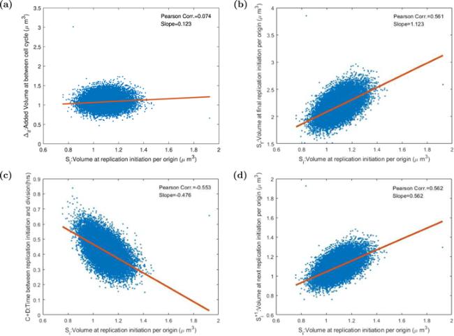
Figure 7. The Pearson correlation coefficients and slopes between various variables in the replication-centric picture. Each point stands for one cell in 20 000 consecutive cells after the system gets into the steady state. The red line is the linear fitting curve. (a) The increment between cell replication cycle Δif is uncorrelated with volume Si at replication initiation per origin. This result certificates the adder property in the replication-centric picture. (b) The correlation coefficient between the volume Si at the initial replication initiation per origin and the volume Sf at the final replication initiation per origin is 0.561 and the slope of the curve 1.123. (c) The time between replication initiation and cell division C + D is negatively correlated with Si. (d) The auto-correlation coefficient of Si is 0.562. If Donchie’s hypothesis is right, the value should be 0. |
4.3. Oscillation of DNA initiation protein expression
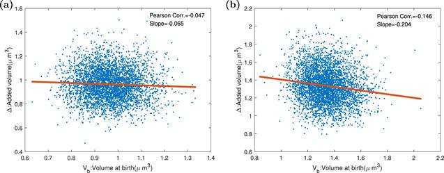
In order to test and verify Amir’s hypothesis [18, 28] that replication and division are regulated together, we set the DNA initiation protein synthesis rate constant to a periodic function with a period 2τ. If replication and division control are co-regulated, as the replication initiation mass changed, the division mass will change in the same direction. A smaller birth size is, a bigger added size generates. The cell will behave like a sizer. But our stochastic simulations do not support co-regulation assumption, and our results confirm the experiment [35] by Si et al. As displayed in figure 8, the oscillation of DNA initiation protein expression does great damage to replication adder, but it does not destroy division adder. Cells in the replication picture are divided into two parts because the oscillation period is twice of division time. Due to the oscillation of synthesis rate, the accumulation time of replication initiation proteins is different, resulting in different replication initiation sizes. Our results imply that the regulations of replication and division are independent, and the division timing is only regulated by division protein.
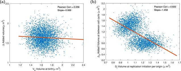
Figure 8. The Pearson correlation coefficients and slopes between birth size, replication initiation size, and added size in the replication-centric picture and division-centric picture when DNA initiation proteins are expressed periodically. Parameters of the dynamics systems are k = 3000 h−1, Σ = 3 ∗ 10−5 μm3 h−1, KD = 4 ∗ 10−12 h−1, KI = $9.2\ast {10}^{-12}\ast | \sin (t\ast \pi /1.446)| /\mathrm{hr}$, dR = dQ = dT = 0.1 h−1, and the other parameters of the model are shown in the table 1. (a) The mean added volume is unchangeable whatever the birth size is, in conflict with co-regulation theory. (b) The periodical oscillation expression of chromosome replication protein changes the initiation mass, destroying the replication adder. |
4.4. Oscillation of division protein expression
In this section, we let the division protein synthesis rate constant oscillate periodically with period 2τ. The production rate of division protein influences the doubling time and division size. Cells are divided into two portions because of different division protein accumulation times. So oscillation of division protein expression ruins the adder property. As shown in figure 9, the replication adder is without affecting. This result indicates that the replication and division control independently. Our results displayed in figures 8 and 9 comply with work [35].
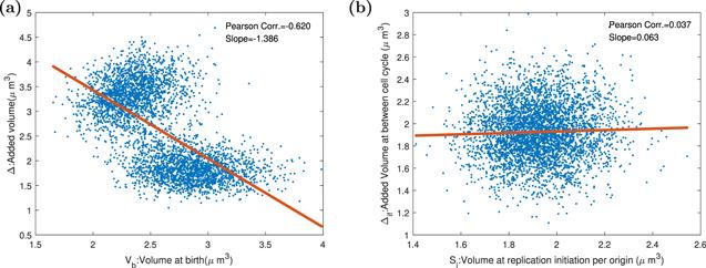
Figure 9. The Pearson correlation coefficients and slopes between birth size, replication initiation size, and added size in the replication-centric picture and division-centric picture when division proteins are expressed periodically. Parameters of the dynamics systems are k = 3000 h−1, Σ = 3 ∗ 10−5 μm3 h−1, ${K}_{D}=4\ast {10}^{-12}\ast | \sin (t\ast \pi /1.446)| /\mathrm{hr}$, KI = 3.4 ∗ 10−12 h−1, dR = dQ = dT = 0.1 h−1, and the other parameters of the model are shown in the table 1. (a) The oscillation of division protein destroys adder property. The smaller the birth size is, the bigger the adder size. (b) DNA replication initiation is not influenced by periodical division protein production, and replication adder is kept. |
4.5. Deviation from adder toward sizer at slow growth rate
It was reported that E.coli exhibited sizer property at slow growth and adder property at fast growth rate [51]. The smaller the birth size is, the bigger the added volume. Why does this phenomenon appear? Si et al [35] hold the viewpoint that the considerable degradation rate of FstZ reduces the auto-correlations of FstZ and division size, and cells deviate to sizer from adder. We made three groups of simulations: no auto-regulation, positive auto-regulation, and negative auto-regulation to confirm the idea. As displayed in figure 10, when the division proteins have a negative auto-regulation and the division protein degradation rate is not zero, cells represent a mildly deviation from adder toward sizer. Besides, when there is no auto-regulation, no deviation from adder will appear. Because of the bistability property of positive auto-regulation, it is possible the division protein synthesis rate is lower than the degradation rate forever. Bistability means that the system has two stable equilibrium states. Under positive feedback, the production rate of division protein is a hill function. The system have three fixed points. The fixed point wherever production rate is equal to degradation rate is unstable. When production rate exceeds degradation rate, division protein will increase, and cell can divide normally. Otherwise division protein will decrease, and cell can’t divide forever. So under the positive auto-regulation condition, there is a considerable probability that cells never divide. It is reasonable to infer that deviation from adder originates from the non-negligible division protein degradation rate.
Figure 10. The Pearson correlation coefficients and the slopes between birth size and added size when division protein degradation rate is zero or not zero, and cells have an auto-inhibition mechanism. Parameters of the dynamics systems are k = 3000 h−1, Σ = 3 ∗ 10−5 μm3 h−1, KD = [200/(200 + d)] ∗ 10−11 h−1, KI = 7 ∗ 10−12 h−1, dR = dQ = dT = 0.1hr−1, and the other parameters of the model are shown in the table 1. (a) The degradation rate of division protein dD is 0. Cells represent adder property. (b) The degradation rate of division protein dD is 1hr−1. Cells slightly deviate from adder property to sizer property. |
5. Discussion
An important issue is how cell counts the trigger protein number or why there is a trigger threshold. In our work, we did not refer to which protein the trigger protein is. In general, the replication protein is thought DNAa. It is reasonable to assume there is a threshold proportional to the origin number. The division protein is always thought FstZ. In the paper [38], authors believe that FstZ amount gets to a threshold proportional to cell diameter, while the diameter of a cell is a constant in a specific growth condition. So it is reasonable to assume there is a threshold to trigger the cell process. There are several cell size regulators, including DNAa, FstZ, and MreB, but we do not have a systematic view on cell size regulation. More experiments to find cell size regulators and more models are needed.
It is weird to suppose trigger proteins degrade or deactivated to a constant [33, 52]. We notice that the two-component model is prevailing in replication initiation and cell division systems [38, 53, 54]. So after the trigger, the trigger proteins turn into the free state from the binding state, and the number of binding state proteins deactivates to a constant.
In our model, every chemical population is proportional to cell volume. But in fact, contents in the membrane proportion is a nonlinear function of cell size. Recent researches [55–57] indicated importance of surface area to volume in the cell size regulation. It is noteworthy that cell wall production is balanced biosynthesis at single-cell level [58]. How cells achieve balanced surface biosynthesis, and the effect of the membrane in cell size regulation are interesting topics.
We did not consider the constraint between KD, KI and Σ, k, so it is not suitable to solve questions in different growth rates. Such as, in the paper [59], authors hold the opinion that the trigger protein production rate is proportional to 1/C, 1/D, or 1/(C + D) where C is the DNA replication time, and D is the time from replication completion to cell division. In future work, it is possible to check SMK growth law and compute the time between replication initiation and cell division in the various growth rates. Whether the DNA replication regulation and division control are interconnected is an interesting question.
Because our work is a self-replication model, the cells grow exponentially. As we know, yeast displays linear growth trajectories [60]. In work [61], authors think linear growth originates from limiting mRNA and DNA. It is valuable to study how cells show non exponential growth and cell size regulation at linear growth.
Cell size noise comes from the stochasticity of chemical reactions, the random partition of cell division, and the fluctuation of single-cell growth rate [47]. We did not consider the growth rate noise. The current model [42, 48] can consider elongation rate noise by dividing cell cycle into many stages. How to combine current model with our model is question worth thinking. Single-cell growth rates do not show linear scaling with respect to the mean [46]. The origin of growth rate noise is unclear, and the influence of growth rate on cell size control is an unanswered question.
6. Conclusion
Altogether, we developed a self-replication model based on work [30, 36, 67], and we added the housekeeping protein and chromosome replication section. We have presented some analytic and numerical results. In the analytical section, we tested Monod growth law. The system we founded evolved to a steady state quickly by our evolution rules and chemical populations, cell size reached homeostasis. By using tens of thousand cells in one evolutionary process, we computed the Pearson correlation coefficient between variables. The correlations have been used to determine which regulation mechanism is adopted by cells. We confirmed the experiment results [34, 35], double-adder mechanism that cells display adder property both in the division cycle and replication cycle. Chromosome replication initiation control is of importance to cell size control because initiation control decides the initiation mass, which determines the unit cell, while the average birth cell size is the sum of unit cells [49]. Although the importance of replication initiation in cell size control, initiation control does not contribute to cell size homeostasis. DNA replication initiation regulation and cell division regulation are independent, and cell division control drives homeostasis regardless of how the chromosome replication initiation is regulated. E.coli at slow growth rate appearing a mildly deviation to sizer from adder is because that the division protein degradation rate is tremendous. In summary, we have implemented a double-adder mechanism in silicon based on two assumptions: (i) there are trigger thresholds for replication initiation and cell division, and after triggering events, the corresponding proteins are degraded to a constant; (ii) chemical populations production rate is proportional to the cell volume, that is, balanced biosynthesis.
Cell size control is valuable to bacterial physiology, and we only know the tip of the iceberg. Understanding the interconnection between cell size regulation, growth rate, division cycle, and replication cycle is complicated and attractive. The reason cells deviate from the adder model is an essential issue for an urgent discussion. A long-term evolution experiment [68, 69] reveals that more giant cells are, a growth rate faster, and the fitness more significant. The relationship between cell size and fitness is worth studying.