


1. Introduction
Recently, the anomalous magnetic moment of the quark [1–10] has attracted much interest in investigating quantum chromodynamic (QCD) matter under a strong magnetic field created through non-central heavy ion collisions [11, 12]. It has been known that the magnetic field catalyzes the chiral condensate of a spin-0 quark–antiquark pair which carries a net magnetic moment and triggers a dynamical anomalous magnetic moment (AMM) of quarks [13–15]. The exact value of a quark's AMM under a magnetic field is unknown but very important for magnetized QCD matter. In this work, we will gain some experience by investigating the AMM of electrons in a magnetic field, which can be calculated from theory and measured experimentally with high precision.
It is well known that a charged fermion can interact with an external magnetic field through an intrinsic magnetic momentum (ℏ = 1, c = 1)
$\begin{eqnarray*}{\boldsymbol{\mu }}=g\left(\displaystyle \frac{q}{2m}\right){\boldsymbol{s}},\end{eqnarray*}$
where q, m, and s are the charge, mass, and spin of the fermion, respectively. For an electron, the $\mathrm{Land}\acute{{\rm{e}}}$ factor ge is believed to be exactly equal to 2 according to Dirac relativistic quantum mechanics. Until a small derivation is observed in an elaborate experiment [16], the deviation of ge from 2 is defined as the anomalous magnetic moment ae = (ge − 2)/2. Meanwhile, quantum electrodynamics (QED) was in its ascendancy and has deepened our understanding of the physical vacuum, where the creation and annihilation of virtual particles contribute additional loop-diagram corrections. The leading order correction ae = α/2π (α ≃ 1/137 is the fine structure constant of QED) calculated by J. Schwinger [17] with renormalizable QED matches the experimental measurement perfectly, powerfully manifesting the validity of quantum field theory.In the standard model, the theoretical contribution to ae comes from three types of interactions, electromagnetic, hadronic, and electroweak:
$\begin{eqnarray*}{a}_{e}(\mathrm{theory})={a}_{e}(\mathrm{QED})+{a}_{e}(\mathrm{hadronic})+{a}_{e}(\mathrm{electroweak}),\end{eqnarray*}$
where the QED contribution can be expressed with perturbative expansion: $\begin{eqnarray*}{a}_{e}(\mathrm{QED})=\sum _{n=1}^{\infty }{\alpha }^{n}{a}_{e}^{(2n)}.\end{eqnarray*}$
J. Schwinger's consequence gives ${a}_{e}^{(2)}=1/2\pi $ and the latest calculation from Aoyama et al [18, 19] has reached up to the tenth-order ${a}_{e}^{(10)}$ with the help of the automatic code generator numerically. The accuracy of experimental electron's AMM ae(experiment) also enhances continually with measurements in a one-electron quantum cyclotron [20–22], which provides us with surprising consistency [19, 22] $\begin{eqnarray*}{a}_{e}(\mathrm{experiment})-{a}_{e}(\mathrm{theory})=-1.06(0.82)\times {10}^{-12}.\end{eqnarray*}$
In essence, the emergence of the electron's AMM is related to slightly broken chiral symmetry because of electron mass me [13], implying any dynamical mechanisms can further break the chiral symmetry always inducing an extra AMM. Naturally, the external magnetic field existing in a one-electron quantum cyclotron is worthy of consideration, for the study of massless spinor QED explicitly shows that a magnetic field reinforces chiral symmetry breaking by endowing the electron with a dynamical mass, known as the magnetic catalysis effect [23], which suggests that the magnetic field could provide an electron with an extra correction. Recently, the latest experimental measurement of muon gμ − 2 confirms the disagreement between experiment and theory [24–28], for the potential possibility as a window to pry into new physics, attracting much attention. All of these motivate us to investigate an electron's AMM in a magnetic field and extend to general fermions, which can deepen our understanding of quantum field theory in a magnetic field.In this work, we investigate the leading order correction of the magnetic field on the AMM of an electron, which can be calculated with relatively high precision. There have been some relevant works to calculate the magnetic correction of an electron by the mass operator and the eigenfunction method [29–32], but these do not consider the Feynman diagram of photon–electron vertex correction as done in usual quantum field theory [33]. The motivation of this work is two-fold: firstly, we would like to check how the magnetic field will modify the AMM of electrons; secondly, the magnetic field dependent on an electron's AMM will shed light on the AMM of quarks under a magnetic field.
2. The leading order correction of electron–photon vertex
The electron-photon coupling in QED is described by ${\rm{i}}{e}\bar{\psi }{\gamma }^{\mu }\psi {A}_{\mu }$. Virtual particle loops provide the vertex with corrections ordered by the order shown in figure 1 by Feynman diagrams:
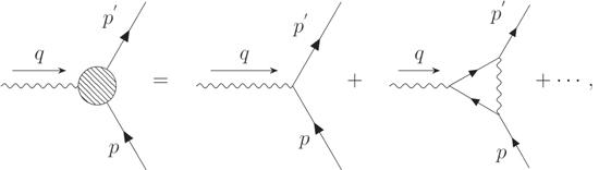
Figure 1. The Feynman diagram of total electron–photon vertex. |
where $q={p}^{{\prime} }-p$ is the momentum transformation and not on-shell q2 ≠ 0, the electromagnetic current changes: $\bar{\psi }{\gamma }^{\mu }\psi \,\longrightarrow \,\bar{\psi }{{\rm{\Gamma }}}^{\mu }\psi $. A complete set of Dirac matrices contain ${{\bf{1}}}_{4\times 4},{\gamma }^{\mu },{\sigma }^{\mu \nu }=\tfrac{{\rm{i}}}{2}[{\gamma }^{\mu },{\gamma }^{\nu }],{\gamma }^{\mu }{\gamma }^{5},{\gamma }^{5}$, the expansion of Γμ in this basis has 16 components. However, the parity symmetry of QED, initial and final electron on-shell, electromagnetic current, and momentum conservation excludes all other terms leaving Γμ in momentum space taking the following form [33]:
$\begin{eqnarray}{{\rm{\Gamma }}}^{\mu }={\gamma }^{\mu }{F}_{1}({q}^{2})+\displaystyle \frac{{\rm{i}}{\sigma }^{\mu \nu }{q}_{\nu }}{2m}{F}_{2}({q}^{2}),\end{eqnarray}$
where m is the electron mass and F1, F2 are form factors and ae(QED) = F2(0) [33]. A point-particle in the absence of radiative corrections has F1 ≡ 1, F2 ≡ 0, which derives the Dirac value for the magnetic moment. Schwinger's calculation of the leading order correction shown in figure 2 gives F2(0) = α/2π, which contributes to the biggest correction.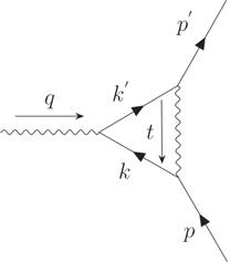
Figure 2. Leading order correction of electron–photon vertex. |
More carefully, the AMM term $\bar{u}({p}^{{\prime} }){\sigma }^{\mu \nu }u(p)$ denotes a helicity-flipping interaction, not invariant under chiral transformation $\psi (x)\to \exp \left({\rm{i}}\theta {\gamma }^{5}\right)\psi (x)$, which indicates the AMM effect emerges from chiral symmetry breaking. Actually, Gordon's identity is derived from the Dirac equation:
$\begin{eqnarray}\begin{array}{l}2m\bar{u}({p}^{{\prime} }){\gamma }^{\mu }u\left(p\right)=\bar{u}({p}^{{\prime} })\\ \,\times \,\left[2{\left({p}^{{\prime} }+p\right)}^{\mu }+{\rm{i}}{\sigma }^{\mu \nu }{q}_{\nu }\right]u\left(p\right),\end{array}\end{eqnarray}$
this formula explicitly exhibits mass term, causing the left-handed fermion to entangle with the right-handed one. If we naively set m = 0, it leads to the massless spinor QED, which is an infrared-free theory, where the photon and electron are not coupled [34], then there will be no observable AMM, i.e., F2 ≡ 0. Nevertheless, this does not conflict with the perturbative and mass-independent consequence F2(0) = α/2π in the one-loop calculation, because QED is not an asymptotically free theory and does not possess a well-defined chiral limit, so the perturbative expression and computation of F2(0) cannot be applied to the case of m = 0. In contrast, the QCD is asymptotically free, whose chiral limit could be rigorously defined nonperturbatively, so a quark's AMM as a continuous function in the chiral limit is expected. This has been confirmed by the Dyson–Schwinger equation calculation [13], which reveals a dressed-quark with a mass of Mq ∼ 0.5 GeV possessing an AMM κq ∝ Mq. In addition, κq ∼ 0.1 is much bigger than an intrinsic one due to the strong breaking of the QCD's chiral symmetry, dramatically changing the nature of quark matter in the magnetic field [10]. The presence of a magnetic field induces a magnetic catalysis effect [35], but it is unknown how this would affect the AMM of quarks. It is quite challenging to do the direct calculation in QCDs because of the nonperturbative nature, therefore we will check the magnetic field-dependent behavior of an electron's AMM and use it for reference in the case of quarks.To calculate the magnetic field correction to the AMM of an electron, we put the Lagrangian density of QED in an external magnetic field,
$\begin{eqnarray}{ \mathcal L }=\bar{\psi }\left({\rm{i}}{\gamma }^{\mu }{D}_{\mu }-m\right)\psi -\displaystyle \frac{1}{4}{F}^{\mu \nu }{F}_{\mu \nu }\end{eqnarray}$
where the covariant derivative ${D}_{\mu }={\partial }_{\mu }-{\rm{i}}e\left({A}_{\mu }^{{\rm{e}}{\rm{x}}{\rm{t}}}+{A}_{\mu }\right)$ and the vector potential ${A}_{\mu }^{{\rm{e}}{\rm{x}}{\rm{t}}}$ introduce an external and uniform magnetic field B = (0, 0, B) along the z direction, we choose the symmetric gauge ${A}_{\mu }^{{\rm{e}}{\rm{x}}{\rm{t}}}=\tfrac{B}{2}(0,y,-x,0)$ for convenience in later calculations. The presence of a magnetic field breaks translation invariance and the amplitude of the process has to be computed in coordinate space and subsequently integrated over space-time [36]. The photon does not carry a charge so the propagator keeps: $\begin{eqnarray}{G}_{\mu \nu }(p)=\displaystyle \frac{-{\rm{i}}{g}_{\mu \nu }}{{p}^{2}+{\rm{i}}\epsilon }.\end{eqnarray}$
For the electron propagator under a uniform magnetic field, the proper-time approach is adopted in coordinate space representation [37]: $\begin{eqnarray}S\left(x,{x}^{{\prime} }\right)={\rm{\Phi }}\left(x,{x}^{{\prime} }\right)\int \displaystyle \frac{{{\rm{d}}}^{4}k}{{\left(2\pi \right)}^{4}}{{\rm{e}}}^{-{\rm{i}}k\cdot \left(x-{x}^{{\prime} }\right)}\tilde{S}(k),\end{eqnarray}$
where $\begin{eqnarray}\begin{array}{l}{\rm{\Phi }}\left(x,{x}^{{\prime} }\right)=\exp \left\{{\rm{i}}\left|q\right|\right.\\ \times \,{\displaystyle \int }_{{x}^{{\prime} }}^{x}{\rm{d}}{\xi }^{\mu }\left.\left[{A}_{\mu }+\displaystyle \frac{1}{2}{F}_{\mu \nu }{\left(\xi -{x}^{{\prime} }\right)}^{\nu }\right]\right\}\end{array}\end{eqnarray}$
is the Schwinger's phase factor, the Fourier transformation of translation invariant part $\tilde{S}(k)$ is given as: $\begin{eqnarray}\begin{array}{l}\tilde{S}(k)={\displaystyle \int }_{0}^{\infty }{\rm{d}}s\,{{\rm{e}}}^{{\rm{i}}s\left({k}_{\parallel }^{2}-{m}^{2}-{k}_{\perp }^{2}\displaystyle \frac{\tan \left(| {qB}| s\right)}{| {qB}| s}+{\rm{i}}\epsilon \right)}\\ \,\times \,\left[\rlap{/}{k}+m+\left({k}^{1}{\gamma }^{2}-{k}^{2}{\gamma }^{1}\right)\tan (| {qB}| s)\right]\\ \,\times \,\left[1-{\gamma }^{1}{\gamma }^{2}\tan (| {qB}| s)\right],\end{array}\end{eqnarray}$
where s is Schwinger's proper-time, the basic notations are defined as: $\begin{eqnarray*}\begin{array}{l}{k}_{\perp }^{\mu }\equiv (0,{k}^{1},{k}^{2},0),\quad {k}_{\parallel }^{\mu }\equiv ({k}^{0},0,0,{k}^{3}),\\ {k}_{\perp }^{2}\equiv {k}_{1}^{2}+{k}_{2}^{2},\quad {k}_{\parallel }^{2}\equiv {k}_{0}^{2}-{k}_{3}^{2},\\ {k}^{2}={k}_{\parallel }^{2}-{k}_{\perp }^{2}.\end{array}\end{eqnarray*}$
Here q represents the charge of the fermion and we assume eB > 0 for convenience.By using the perturbative method, we can expand the total vertex amplitude with respect to α in leading-order
$\begin{eqnarray}\begin{array}{l}\bar{u}({p}^{{\prime} }){{\rm{\Gamma }}}^{\mu }u(p)=\bar{u}({p}^{{\prime} }){\gamma }^{\mu }u(p)\\ \,+\,\bar{u}({p}^{{\prime} }){{ \mathcal M }}^{\mu }u(p)+{ \mathcal O }(\alpha ).\end{array}\end{eqnarray}$
As is shown in figure 2, the leading-order correction ${{ \mathcal M }}^{\mu }$ reads: $\begin{eqnarray}\begin{array}{l}{{ \mathcal M }}^{\mu }=\displaystyle \int {{\rm{d}}}^{4}x{{\rm{d}}}^{4}y{{\rm{d}}}^{4}z\,{\rm{\Phi }}(x,y){\rm{\Phi }}(y,z)\\ \displaystyle \int \displaystyle \frac{{{\rm{d}}}^{4}t}{{\left(2\pi \right)}^{4}}\displaystyle \frac{{{\rm{d}}}^{4}{k}^{{\prime} }}{{\left(2\pi \right)}^{4}}\displaystyle \frac{{{\rm{d}}}^{4}k}{{\left(2\pi \right)}^{4}}\\ \times \,{{\rm{e}}}^{-{\rm{i}}t\cdot (z-x)}{{\rm{e}}}^{-{\rm{i}}k\cdot (x-y)}{{\rm{e}}}^{-{\rm{i}}{k}^{{\prime} }\cdot (y-z)}{{\rm{e}}}^{{\rm{i}}p\cdot x}{{\rm{e}}}^{{\rm{i}}q\cdot y}{{\rm{e}}}^{-{\rm{i}}{p}^{{\prime} }\cdot z}{G}_{\nu \rho }(t)\\ \times \,(-{\rm{i}}e{\gamma }^{\nu })\tilde{S}({k}^{{\prime} }){\gamma }^{\mu }\tilde{S}(k)(-{\rm{i}}e{\gamma }^{\rho }),\\ =\,\displaystyle \int \displaystyle \frac{{{\rm{d}}}^{4}t}{{\left(2\pi \right)}^{4}}\displaystyle \frac{{{\rm{d}}}^{4}{k}^{{\prime} }}{{\left(2\pi \right)}^{4}}\displaystyle \frac{{{\rm{d}}}^{4}k}{{\left(2\pi \right)}^{4}}\times \displaystyle \frac{{\rm{i}}{e}^{2}}{{t}^{2}}\\ \times \,{\displaystyle \int }_{0}^{\infty }{\rm{d}}r{\displaystyle \int }_{0}^{\infty }{\rm{d}}s{{\rm{e}}}^{{\rm{i}}r\left({k}_{\parallel }^{{\prime} 2}-{m}^{2}-{k}_{\perp }^{{\prime} 2}\displaystyle \frac{\tan \left({eBr}\right)}{{eBr}}\right)}{{\rm{e}}}^{{\rm{i}}s\left({k}_{\parallel }^{2}-{m}^{2}-{k}_{\perp }^{2}\displaystyle \frac{\tan \left({eBr}\right)}{{eBs}}\right)}\\ \times \,{\gamma }^{\nu }\left[{\rlap{/}{k}}^{{\prime} }+m+\left({k}^{{\prime} 1}{\gamma }^{2}-{k}^{{\prime} 2}{\gamma }^{1}\right)\tan ({eBr})\right]\left[1-{\gamma }^{1}{\gamma }^{2}\right.\\ \times \,\left.\tan ({eBr})\right]{\gamma }^{\mu }\\ \times \,\left[\rlap{/}{k}+m+\left({k}^{1}{\gamma }^{2}-{k}^{2}{\gamma }^{1}\right)\tan ({eBs})\right]\left[1-{\gamma }^{1}{\gamma }^{2}\tan ({eBs})\right]{\gamma }_{\nu }\\ \times \,\displaystyle \int {{\rm{d}}}^{4}x{{\rm{d}}}^{4}y{{\rm{d}}}^{4}z\,{\rm{\Phi }}(x,y){\rm{\Phi }}(y,z){{\rm{e}}}^{-{\rm{i}}t\cdot (z-x)}{{\rm{e}}}^{-{\rm{i}}k\cdot (x-y)}\\ \times \,{{\rm{e}}}^{-{\rm{i}}{k}^{{\prime} }\cdot (y-z)}{{\rm{e}}}^{{\rm{i}}p\cdot x}{{\rm{e}}}^{{\rm{i}}q\cdot y}{{\rm{e}}}^{-{\rm{i}}{p}^{{\prime} }\cdot z},\end{array}\end{eqnarray}$
where x, y, z are the three space-time vertexes with corresponding momentum, s, r and Φ(x, y), Φ(y, z) are proper-time and phase factors emerging from two-electron propagators. The expression of ${{ \mathcal M }}^{\mu }$ is quite tedious, in the following we separate ${{ \mathcal M }}^{\mu }$ into three parts: 1) the phase factor $P(t,k,{k}^{{\prime} })$, 2) the momentum integral ${ \mathcal I }$, and 3) the γ matrix part Θμ(r, s) with their explicit expressions given below: $\begin{eqnarray}\begin{array}{l}P(t,k,{k}^{{\prime} })=\displaystyle \int {{\rm{d}}}^{4}x{{\rm{d}}}^{4}y{{\rm{d}}}^{4}z\,{\rm{\Phi }}(x,y){\rm{\Phi }}(y,z)\\ \,\times \,\,{{\rm{e}}}^{-{\rm{i}}t\cdot (z-x)}{{\rm{e}}}^{-{\rm{i}}k\cdot (x-y)}{{\rm{e}}}^{-{\rm{i}}{k}^{{\prime} }\cdot (y-z)}{{\rm{e}}}^{{\rm{i}}p\cdot x}{{\rm{e}}}^{{\rm{i}}q\cdot y}{{\rm{e}}}^{-{\rm{i}}{p}^{{\prime} }\cdot z},\end{array}\end{eqnarray}$
$\begin{eqnarray}\begin{array}{l}{ \mathcal I }=\displaystyle \int \displaystyle \frac{{{\rm{d}}}^{4}t}{{\left(2\pi \right)}^{4}}\displaystyle \frac{{{\rm{d}}}^{4}{k}^{{\prime} }}{{\left(2\pi \right)}^{4}}\displaystyle \frac{{{\rm{d}}}^{4}k}{{\left(2\pi \right)}^{4}}P(t,k,{k}^{{\prime} })\\ \,\times \,\displaystyle \frac{{\rm{i}}{e}^{2}}{{t}^{2}}{\displaystyle \int }_{0}^{\infty }{\rm{d}}r{\displaystyle \int }_{0}^{\infty }{\rm{d}}s{{\rm{e}}}^{{\rm{i}}r\left({k}_{\parallel }^{{\prime} 2}-{m}^{2}-{k}_{\perp }^{{\prime} 2}\displaystyle \frac{\tan \left({eBr}\right)}{{eBr}}\right)}\\ \,\times \,{{\rm{e}}}^{{\rm{i}}s\left({k}_{\parallel }^{2}-{m}^{2}-{k}_{\perp }^{2}\displaystyle \frac{\tan \left({eBr}\right)}{{eBs}}\right)}\end{array}\end{eqnarray}$
$\begin{eqnarray}\begin{array}{l}{{\rm{\Theta }}}^{\mu }(r,s)={\gamma }^{\nu }\left[{\rlap{/}{k}}^{{\prime} }+m+\left({k}^{{\prime} 1}{\gamma }^{2}-{k}^{{\prime} 2}{\gamma }^{1}\right)\tan ({eBr})\right]\\ \times \,\left[1-{\gamma }^{1}{\gamma }^{2}\tan ({eBr})\right]{\gamma }^{\mu }\\ \times \,\left[\rlap{/}{k}+m+\left({k}^{1}{\gamma }^{2}-{k}^{2}{\gamma }^{1}\right)\tan ({eBs})\right]\\ \times \,\left[1-{\gamma }^{1}{\gamma }^{2}\tan ({eBs})\right]{\gamma }_{\nu }.\end{array}\end{eqnarray}$
In the next subsections, we will carefully handle these three parts, respectively.2.1. The phase factor part
In this section, we deal with the Schwinger part $P(t,k,{k}^{{\prime} })$. With the symmetric gauge ${A}^{\mu }=\tfrac{B}{2}(0,-y,x,0)$ and equation (6 ), the only non-zero terms of Fμν are F12 = − F21 = − B , so the product of the phase factor can be written asA . It is worth mentioning that the longitudinal momentum is strictly conserved but the transverse momentum expresses a distribution function. The magnetic field causes dimension reduction leaving the longitudinal physics unchanged but the transverse remains a little subtle. Now ${{ \mathcal M }}^{\mu }$ becomes:15 ), so the momentum conservation conditions: ${t}_{\parallel }={k}_{\parallel }-{p}_{\parallel },{k}_{\parallel }^{{\prime} }={k}_{\parallel }+{q}_{\parallel }$ become ${t}_{\parallel }={k}_{\parallel },{k}_{\parallel }^{{\prime} }={k}_{\parallel }$.
$\begin{eqnarray}\begin{array}{l}{\rm{\Phi }}(x,y){\rm{\Phi }}(y,z)={{\rm{e}}}^{{\rm{i}}\cdot \displaystyle \frac{{eB}}{2}({\epsilon }_{{ij}}{x}^{j}{y}^{i}+{\epsilon }_{{ij}}{y}^{j}{z}^{i})}\\ \,=\,{{\rm{e}}}^{{\rm{i}}\cdot \displaystyle \frac{{eB}}{2}{\epsilon }_{{ij}}{y}^{i}{\left(x-z\right)}^{j}}.\end{array}\end{eqnarray}$
Introducing a variable h = x − z, one has x = h + z, d4x = d4h and after the integration of the space-time, we have: $\begin{eqnarray}\begin{array}{l}P(t,k,{k}^{{\prime} })=\displaystyle \int {{\rm{d}}}^{4}x{{\rm{d}}}^{4}y{{\rm{d}}}^{4}z\,{\rm{\Phi }}(x,y){\rm{\Phi }}(y,z){{\rm{e}}}^{-{\rm{i}}t\cdot (z-x)}{{\rm{e}}}^{-{\rm{i}}k\cdot (x-y)}\\ \,\times \,{{\rm{e}}}^{-{\rm{i}}{k}^{{\prime} }\cdot (y-z)}{{\rm{e}}}^{{\rm{i}}p\cdot x}{{\rm{e}}}^{{\rm{i}}q\cdot y}{{\rm{e}}}^{-{\rm{i}}{p}^{{\prime} }\cdot z}\\ =\,{\left(2\pi \right)}^{2}4{l}^{4}{{\rm{e}}}^{-{\rm{i}}\cdot 2{\left(p+t-k\right)}^{1}{\left(q+k-{k}^{{\prime} }\right)}_{2}/| {eB}| }\\ \,\times \,{{\rm{e}}}^{{\rm{i}}\cdot 2{\left(p+t-k\right)}^{2}{\left(q+k-{k}^{{\prime} }\right)}_{1}/| {eB}| }\\ \,\times \,{\left(2\pi \right)}^{4}{\delta }^{4}(p-k+{k}^{{\prime} }-{p}^{{\prime} }){\left(2\pi \right)}^{2}\\ \,\times \,{\delta }^{2}({p}_{\parallel }+{t}_{\parallel }-{k}_{\parallel }){\left(2\pi \right)}^{2}{\delta }^{2}({q}_{\parallel }+{k}_{\parallel }-{k}_{\parallel }^{{\prime} }),\end{array}\end{eqnarray}$
where $l=1/\sqrt{| {eB}| }$ is the magnetic length. More details of this calculation are featured in appendix $\begin{eqnarray}\begin{array}{c}{{ \mathcal M }}^{\mu }=\displaystyle \int ({\rm{d}}{t}_{\perp }{\rm{d}}{k}_{\perp }^{{\prime} }{\rm{d}}k){\left(2\pi \right)}^{2}{\delta }^{2}({p}_{\parallel }^{{\prime} }-{p}_{\parallel }-{q}_{\parallel })\\ \times \,{\left(2\pi \right)}^{2}{\delta }^{2}({p}_{\perp }-{k}_{\perp }-{p}_{\perp }^{{\prime} }+{k}_{\perp }^{{\prime} })\\ \times \,{\left(2\pi \right)}^{2}4{l}^{4}{{\rm{e}}}^{-{\rm{i}}\cdot 2{\left(p+t-k\right)}^{1}{\left(q+k-{k}^{{\prime} }\right)}_{2}/| {eB}| }\\ \times \,{{\rm{e}}}^{{\rm{i}}\cdot 2{\left(p+t-k\right)}^{2}{\left(q+k-{k}^{{\prime} }\right)}_{1}/| {eB}| }\times {{ \mathcal A }}^{\mu }(t,k,{k}^{{\prime} })\\ ={\rm{\Delta }}\displaystyle \int ({\rm{d}}{t}_{\perp }{\rm{d}}{k}_{\perp }^{{\prime} }{\rm{d}}k){\left(2\pi \right)}^{2}4{l}^{4}{{\rm{e}}}^{-{\rm{i}}\cdot 2{\left(t-k\right)}^{1}{\left(k-{k}^{{\prime} }\right)}_{2}/| {eB}| }\\ \times \,{{\rm{e}}}^{{\rm{i}}\cdot 2{\left(t-k\right)}^{2}{\left(k-{k}^{{\prime} }\right)}_{1}/| {eB}| }\times {{ \mathcal A }}^{\mu }(t,k,{k}^{{\prime} }),\end{array}\end{eqnarray}$
where $\begin{eqnarray}\begin{array}{l}{\rm{\Delta }}={\left(2\pi \right)}^{2}{\delta }^{2}({p}_{\parallel }^{{\prime} }-{p}_{\parallel }-{q}_{\parallel }){\left(2\pi \right)}^{2}\\ \times \,{\delta }^{2}\left({p}_{\perp }-{k}_{\perp }-{p}_{\perp }^{{\prime} }+{k}_{\perp }^{{\prime} }\right)\end{array}\end{eqnarray}$
and $\begin{eqnarray}\begin{array}{l}{{ \mathcal A }}^{\mu }(t,k,{k}^{{\prime} })={G}_{\nu \rho }(t)(-{\rm{i}}e{\gamma }^{\nu })\tilde{S}({k}^{{\prime} }){\gamma }^{\mu }\tilde{S}(k)(-{\rm{i}}e{\gamma }^{\rho })\\ =\,\displaystyle \frac{{\rm{i}}{e}^{2}}{{t}^{2}}{\displaystyle \int }_{0}^{\infty }{\rm{d}}r{\displaystyle \int }_{0}^{\infty }{\rm{d}}s\\ \times \,{{\rm{e}}}^{{\rm{i}}r\left({k}_{\parallel }^{{\prime} 2}-{m}^{2}-{k}_{\perp }^{{\prime} 2}\displaystyle \frac{\tan \left({eBr}\right)}{{eBr}}\right)}\\ \times \,{{\rm{e}}}^{{\rm{i}}s\left({k}_{\parallel }^{2}-{m}^{2}-{k}_{\perp }^{2}\displaystyle \frac{\tan \left({eBr}\right)}{{eBs}}\right)}\times {{\rm{\Theta }}}^{\mu }(r,s),\end{array}\end{eqnarray}$
with $({\rm{d}}k)\equiv \tfrac{{{\rm{d}}}^{4}k}{{\left(2\pi \right)}^{4}},({\rm{d}}{k}_{\perp })\equiv \tfrac{{{\rm{d}}}^{2}{k}_{\perp }}{{\left(2\pi \right)}^{2}},({\rm{d}}{k}_{\parallel })\equiv \tfrac{{{\rm{d}}}^{2}{k}_{\parallel }}{{\left(2\pi \right)}^{2}}$ for simplification. The AMM is defined when q is very small and the measurement of AMM proceeds in a low-energy condition, which suggests a reasonable approximation: q → 0, p → 0 applied in the last line of equation (2.2. The momentum integral part
Actually, the AMM part ${{\rm{\Theta }}}_{\mathrm{AMM}}^{\mu }$ can be extracted from Θμ(r, s) later and irrelevant to the momenta $t,k,{k}^{{\prime} }$, we can integrate all three momenta in equation (15 ), which exactly results in integral part ${ \mathcal I }$ :B . Finally, we obtain a much more transparent expression:
$\begin{eqnarray}\begin{array}{l}{ \mathcal I }={\left(2\pi \right)}^{2}4{l}^{4}{\displaystyle \int }_{0}^{\infty }{\rm{d}}r{\displaystyle \int }_{0}^{\infty }{\rm{d}}s\\ \,\times \,\displaystyle \int ({\rm{d}}{t}_{\perp }{\rm{d}}{k}_{\perp }^{{\prime} }{\rm{d}}k)\displaystyle \frac{{\rm{i}}{e}^{2}}{{k}_{\parallel }^{2}-{t}_{\perp }^{2}}\\ \,\times \,{{\rm{e}}}^{-{\rm{i}}\cdot 2{\left(t-k\right)}^{1}{\left(k-{k}^{{\prime} }\right)}_{2}/| {eB}| }{{\rm{e}}}^{{\rm{i}}\cdot 2{\left(t-k\right)}^{2}{\left(k-{k}^{{\prime} }\right)}_{1}/| {eB}| }\\ \,\times \,{{\rm{e}}}^{{\rm{i}}r\left({k}_{\parallel }^{2}-{m}^{2}-{k}_{\perp }^{{\prime} 2}\displaystyle \frac{\tan \left({eBr}\right)}{{eBr}}\right)}{{\rm{e}}}^{{\rm{i}}s\left({k}_{\parallel }^{2}-{m}^{2}-{k}_{\perp }^{2}\displaystyle \frac{\tan \left({eBr}\right)}{{eBs}}\right)},\end{array}\end{eqnarray}$
where ${t}^{2}={k}_{\parallel }^{2}-{t}_{\perp }^{2}$ by momentum conservation. In order to remove the pole of momentum integral, we do a Wick rotation transferring Minkowski space-time into a Euclidean one [23]: k0 → ik0, r → − ir, s → − is. So the integral becomes $\begin{eqnarray}\begin{array}{c}{ \mathcal I }={\left(2\pi \right)}^{2}4{l}^{4}\times {\left(-{\rm{i}}\right)}^{2}{\displaystyle \int }_{0}^{\infty }{\rm{d}}r{\displaystyle \int }_{0}^{\infty }{\rm{d}}s\\ \times \left({\rm{i}}\right)\displaystyle \int ({{\rm{d}}t}_{\perp }{{\rm{d}}k}_{\perp }^{{\prime} }{{\rm{d}}k}_{E})\displaystyle \frac{-{\rm{i}}{e}^{2}}{{k}_{\parallel E}^{2}+{t}_{\perp }^{2}}\\ \times {{\rm{e}}}^{\left.-{\rm{i}}\cdot 2{\left(t-k\right)}^{1}{\left(k-{k}^{{\prime} }\right)}_{2}/| {eB}\right|}{{\rm{e}}}^{{\rm{i}}\cdot 2{\left(t-k\right)}^{2}{\left(k-{k}^{{\prime} }\right)}_{1}/| {eB}| }\\ \times \, \ {{\rm{e}}}^{-r\left({k}_{\parallel E}^{2}\ +\ {m}^{2}\right)-{k}_{\perp }^{{\prime} 2}\ {l}^{2}\tanh \left({eBr}\right)}\\ \times \,{{\rm{e}}}^{-s\left({k}_{\parallel E}^{2}\ +\ {m}^{2}\right)-{k}_{\perp }^{2}\ {l}^{2}\tanh \left({eBs}\right)},\end{array}\end{eqnarray}$
here, we use $\tan (-{\rm{i}}x)=-\mathrm{itanh}(x),{k}_{\parallel E}={k}_{0}^{2}+{k}_{3}^{2}$, the integral about proper-time r or s, momentum k0 and photon propagator contribute −i, i, −1 under Wick rotation, respectively. Even in Euclidean space, the integral calculation is still tedious and complicated, therefore we put all details of this calculation in appendix $\begin{eqnarray}\begin{array}{l}{ \mathcal I }=-\displaystyle \frac{\alpha }{4\pi {l}^{2}}{\displaystyle \int }_{0}^{\infty }{\displaystyle \int }_{0}^{\infty }{\rm{d}}r{\rm{d}}s\\ \,\times \,\displaystyle \frac{{{\rm{e}}}^{-(r+s){m}^{2}}}{\left[\tanh ({eBr})+\tanh ({eBs})\right]}\displaystyle \frac{\mathrm{ln}v}{v-1}\end{array}\end{eqnarray}$
with fine structure constant α = e2/4π and $v=({eBr}+{eBs})/\tanh ({eBr}+{eBs})$ .2.3. The AMM term extracted from Θμ(r, s)
The presence of the magnetic field breaks the original parity symmetry, thus the leading-order vertex structure equation (12 ) becomes more complicated than the original one in equation (1 ). Fortunately, we just need to extract and calculate the term related to the AMM and to not get stuck in the swamp of total Θμ(r, s). As is seen in equation (1 ), the linear term of q corresponds to the AMM effect in absence of a magnetic field. We naturally have the momentum constraint in the longitudinal direction ${q}_{\parallel }={k}_{\parallel }^{{\prime} }-{k}_{\parallel }$ which helps to separate the linear term of q but the momentum constraint in the transverse direction emerges as a distribution function equation (14 ). Therefore, it is impossible to have the same definition of AMM as in the vacuum, but considering the phase factor equation (14 ) is a highly oscillating function in a weak magnetic field region, this indicates that the momentum ${q}_{\perp }={k}_{\perp }^{{\prime} }-{k}_{\perp }$ substantially dominates the distribution. So under the approximation ${q}_{\perp }\simeq {k}_{\perp }^{{\prime} }-{k}_{\perp }$, the linear part of q in Θμ can be subtracted and takes the following form:
$\begin{eqnarray}\begin{array}{l}{{\rm{\Theta }}}^{\mu }{\left(r,s\right)}_{q-\mathrm{linear}}={\gamma }^{\nu }\rlap{/}{\tilde{q}}\left[1-{\gamma }^{1}{\gamma }^{2}\tan ({eBr})\right]{\gamma }^{\mu }\\ \,\times \,\left[\rlap{/}{k}+m+\left({k}^{1}{\gamma }^{2}-{k}^{2}{\gamma }^{1}\right)\tan ({eBs})\right]\\ \,\times \,\left[1-{\gamma }^{1}{\gamma }^{2}\tan ({eBs})\right]{\gamma }_{\nu },\end{array}\end{eqnarray}$
where $\tilde{q}=q+\hat{q},\hat{q}:= \left(0,{q}_{2}\tan ({eBr}),-{q}_{1}\tan ({eBr}),0\right)$. It is noticed that only the terms consisting of the product of even γ matrices contribute to the AMM, thus we directly get rid of other terms and obtain: $\begin{eqnarray}\begin{array}{l}{{\rm{\Theta }}}^{\mu }{\left(r,s\right)}_{\mathrm{AMM}}={\gamma }^{\nu }\rlap{/}{\tilde{q}}\left[1-{\gamma }^{1}{\gamma }^{2}\tan ({eBr})\right]\\ \,\times \,{\gamma }^{\mu }m\left[1-{\gamma }^{1}{\gamma }^{2}\tan ({eBs})\right]{\gamma }_{\nu }\\ =\,m{\gamma }^{\nu }\rlap{/}{\tilde{q}}\left[{\gamma }^{\mu }-{\gamma }^{\mu }{\gamma }^{1}{\gamma }^{2}\tan ({eBs})\right.\\ \,-\,{\gamma }^{1}{\gamma }^{2}{\gamma }^{\mu }\tan ({eBr})\\ \,\times \,\left.+\,{\gamma }^{1}{\gamma }^{2}{\gamma }^{\mu }{\gamma }^{1}{\gamma }^{2}\tan ({eBr})\tan ({eBs})\right]{\gamma }_{\nu }.\end{array}\end{eqnarray}$
The presence of the magnetic field creates anisotropy between the x − y plane and z direction so that the AMM correction becomes different in the longitudinal and transverse directions. While a magnetic field along the z axis is imposing, the classical interaction term − μ · B, μ = (μx, μy, μz) implies only μz is measurable, corresponding to μ = 1, 2 components of the magnetic vector potential Aμ. Thus the magnetic interaction amplitude is given by $\begin{eqnarray}\begin{array}{l}\bar{u}({p}^{{\prime} }){{ \mathcal M }}^{i}u(p){\tilde{A}}^{i}=\bar{u}({p}^{{\prime} }){{ \mathcal M }}^{1}u(p){\tilde{A}}^{1}\\ \,+\,\bar{u}({p}^{{\prime} }){{ \mathcal M }}^{2}u(p){\tilde{A}}^{2}\end{array}\end{eqnarray}$
where ${\tilde{A}}^{\mu }$ is the Fourier transformation of Aμ, which guides us to concentrate on Θμ with μ = 1, 2 components. Because two transverse directions share the same physics, therefore we just need to display the case μ = 1.When μ = 1, we can simplify the expression into a more friendly form by the Dirac algebra:1 ) in the vacuum. From the above-complicated expression, it is difficult to read explicit information about the magnetic correction of the AMM term.
$\begin{eqnarray}\begin{array}{l}{{\rm{\Theta }}}^{1}{\left(r,s\right)}_{\mathrm{AMM}}=\displaystyle \frac{{\rm{i}}{\sigma }^{1\alpha }{q}_{\alpha }}{2m}\{-8{m}^{2}\left[1+\tan ({eBr})\tan ({eBs})\right]\}\\ +\,\displaystyle \frac{{\rm{i}}{\sigma }^{2\alpha }{q}_{\alpha }}{2m}\{-8{m}^{2}\left[\tan ({eBs})-\tan ({eBr})\right]\}\\ +\,\displaystyle \frac{{\rm{i}}{\sigma }^{1\alpha }{\hat{q}}_{\alpha }}{2m}\{-8{m}^{2}\left[1+\tan ({eBr})\tan ({eBs})\right]\}\\ +\,\displaystyle \frac{{\rm{i}}{\sigma }^{2\alpha }{\hat{q}}_{\alpha }}{2m}\{-8{m}^{2}\left[\tan ({eBs})-\tan ({eBr})\right]\}\\ +\,4m\rlap{/}{q}\left[{\gamma }^{1}+{\gamma }^{2}\tan ({eBs})-{\gamma }^{2}\tan ({eBr})\right.\\ \left.+\,{\gamma }^{1}\tan ({eBr})\tan ({eBs})\right]\\ +\,4m\rlap{/}{\hat{q}}\left[{\gamma }^{1}+{\gamma }^{2}\tan ({eBs})-{\gamma }^{2}\tan ({eBr})\right.\\ \left.+\,{\gamma }^{1}\tan ({eBr})\tan ({eBs})\right].\end{array}\end{eqnarray}$
The presence of the magnetic field breaks the concise structure of the electron-photon vertex equation (Comparing with equation (1 ), we find the first term of equation (24 ) possesses the standard form contributing to the magnetic correction of AMM [33], but the other terms are more veiled, whose physical meaning will be explained by seeking the corresponding non-relativistic limit analyzed in appendix C . Finally, the last line also contributes corrections to AMM. Extracting the coefficient of the total magnetic correction term of the electron in equation (24 ) gives
$\begin{eqnarray}8{m}^{2}\left[{\tan }^{2}({eBr})-2\tan ({eBr})\tan ({eBs})\right].\end{eqnarray}$
Some non-invariant terms under gauge transformation that cannot present observable phenomena are neglected.3. Conclusion and discussion
For a measurable AMM correction, we only need to calculate the major contribution of ${{ \mathcal M }}^{\mu }$ in the x, y direction. Extracting the relevant term from equation (24 ) and doing a Wick rotation r → − ir, s → − is,20 ) obtaining the magnetic correction to the AMM of the electron:27 ) do not keep symmetric as in equation (20 ) due to the presence of the magnetic field. As such, the time reversal invariance no longer maintains as QED in the vacuum, so the two parameters r, s, corresponding propagators with a time order, have different positions. Moreover, we see that the final expression of κB manifesting the magnetic correction is negative prompting us to check where the minus sign originates. Let us recall the equation (19 ), there are two electron propagators, one photon propagator, two vertex, respectively, contributing ${\left(-{\rm{i}}\right)}^{2}$, − i × ( − 1), ${\left(-{\rm{i}}\right)}^{2}$ after Wick rotation with an extra i in differential dk, which results in a minus sign ${\left(-{\rm{i}}\right)}^{2}\times {\rm{i}}\times {\left(-{\rm{i}}\right)}^{2}\times {\rm{i}}=-1$. Here, we would like to point out that the result in equation (27 ) vanishes when eB=0 so cannot continuously go back to the Schwinger result ${a}_{e}=\tfrac{\alpha }{2\pi }$ , one can regard this magnetic correction as an extra contribution from the magnetic field. After taking the vacuum contribution into consideration, the leading order correction to AMM of the electron is:
$\begin{eqnarray}\begin{array}{l}8{m}^{2}\left[{\tan }^{2}({eBr})-2\tan ({eBr})\tan ({eBs})\right]\\ \,\longrightarrow \ 8{m}^{2}\left[2\tanh ({eBr})\tanh ({eBs})-{\tanh }^{2}({eBr})\right].\end{array}\end{eqnarray}$
Therefore, one multiplies the meaningful part with integral ${ \mathcal I }$ in equation ( $\begin{eqnarray}\begin{array}{l}{\kappa }_{B}=-\displaystyle \frac{4{m}^{2}\alpha }{2\pi {l}^{2}}{\displaystyle \int }_{0}^{\infty }{\displaystyle \int }_{0}^{\infty }{{\rm{e}}}^{-(r+s){m}^{2}}\\ \,\times \,\displaystyle \frac{\left[2\tanh ({eBr})\tanh ({eBs})-{\tanh }^{2}({eBr})\right]}{\left[\tanh ({eBr})+\tanh ({eBs})\right]}\displaystyle \frac{\mathrm{ln}v}{v-1}{\rm{d}}r{\rm{d}}s\\ =\,-\displaystyle \frac{4{m}^{2}{l}^{2}\alpha }{2\pi }{\displaystyle \int }_{0}^{\infty }{\displaystyle \int }_{0}^{\infty }{{\rm{e}}}^{-(R+S){m}^{2}{l}^{2}}\\ \,\times \,\displaystyle \frac{\left[2\tanh (R)\tanh (S)-{\tanh }^{2}(R)\right]}{\left[\tanh (R)+\tanh (S)\right]}\displaystyle \frac{\mathrm{ln}V}{V-1}{\rm{d}}R{\rm{d}}S\end{array}\end{eqnarray}$
with $v=\tfrac{{eBr}+{eBs}}{\tanh ({eBr}+{eBs})},V=\tfrac{R\,+\,S}{\tanh (R+S)},l=1/\sqrt{| {eB}| }$, and variable transformations R = eBr, S = eBs done. First of all, there is one very interesting point that two parameters r, s (or R, S) in equation ( $\begin{eqnarray}\begin{array}{l}{a}_{e}=\displaystyle \frac{\alpha }{2\pi }+{\kappa }_{B},\\ =\,\displaystyle \frac{\alpha }{2\pi }\left(1-4{m}^{2}{l}^{2}{\displaystyle \int }_{0}^{\infty }{\displaystyle \int }_{0}^{\infty }{{\rm{e}}}^{-(R+S){m}^{2}{l}^{2}}\right.\\ \,\times \,\left.\displaystyle \frac{\left[2\tanh (R)\tanh (S)-{\tanh }^{2}(R)\right]}{\left[\tanh (R)+\tanh (S)\right]}\displaystyle \frac{\mathrm{ln}V}{V-1}{\rm{d}}R{\rm{d}}S\right).\end{array}\end{eqnarray}$
Analytically, m2l2 is the only dimensionless combination with eB, m, which appears twice in the expression: 1) 4m2l2 as a coefficient in front of the whole expression confirms that the magnetic correction to AMM κB ∝ m2, which indicates that the magnetic correction is a nonperturbative contribution similar to the AMM induced by the chiral symmetry breaking [13–15]. This also naturally explains why the magnetic correction results cannot smoothly go back to $\tfrac{\alpha }{2\pi }$ when eB=0. The nonperturbative nature of chiral symmetry breaking induced by a constant magnetic field was also been discussed in the 1990s [38–41]. 2)m2l2 appears in the exponential factor which strongly depresses the integral so that the correction κB will only become considerable when $\sqrt{{eB}}\sim m$.For the magnetic field magnitude B ∼ 1 T ↔ eB ∼ 2 × 10⁻¹⁰MeV2 used in the laboratory to measure the electron g − 2, ∣κB∣ < 10−33, is much smaller than the measurement ae = 0.00115965218073(28) [22, 24]. For the muon, whose mass is much heavier than the electron ${\left({m}_{\mu }/{m}_{e}\right)}^{2}=43000$, under the same magnetic field magnitude B ∼ 1 T ↔ eB ∼ 2 × 10⁻¹⁰MeV2, we find that the corresponding magnetic correction to the AMM is ∣κB∣ < 10−42, which is also much smaller than the experimental measurement of muon aμ = 0.00116592040(54) [24]. Thus one can safely neglect the magnetic correction to the AMM of the electron/muon in the vacuum.
The magnetic correction κB will become considerable when $\sqrt{{eB}}\sim m$, which can be seen explicitly from the numerical result shown in figure (3) on the magnetic correction κB in equation (27 ) to the electron and muon as a function of $\sqrt{{eB}}/m$ with m = me and m = mμ. To see how the negative magnetic correction κB affects physics, we consider the electron or a fermion with AMM κ + κB travels in the magnetic field, one can derive its dispersion as below:
$\begin{eqnarray}{E}_{l,s}^{2}=\left\{\begin{array}{ll}{p}_{z}^{2}+{\left[\sqrt{{m}^{2}+\left(2l+1+s\right)| {eB}| }-s(\kappa +{\kappa }_{B}){eB}\right]}^{2}, & l\geqslant 1.\\ {p}_{z}^{2}+{[m-(\kappa +{\kappa }_{B}){eB}]}^{2}, & l=0.\end{array}\right.\end{eqnarray}$
where l, s = ± 1 are quantum numbers of orbital and spin angular momentum, respectively, eB > 0 for convenience. As is seen, the normal AMM κ causes the splitting of degenerate energy levels known as the Zeeman effect in the spectrum, which is used in the accurate measurement of the AMM [18, 19]. However, the energy level splitting will be suppressed with a negative magnetic correction taken into account κ → κ + κB, which will lead to a slight diamagnetism. κB increases the energy of the system expressing a trivial magnetic catalysis effect as usual [23]. We will explicitly show these properties in a separate paper [42]. Actually, our calculation mainly concentrates on the leading order correction to the AMM of the electron, the next to leading order and higher orders should also contribute to the correction, but the small coupling of QED $\alpha \sim { \mathcal O }(1/100)$ guarantees that we can safely ignore higher-order influence. Moreover, due to the vacuum polarization, the photon with a mass ${M}_{\gamma }^{2}\sim { \mathcal O }(\alpha | {eB}| )$ results in a very strong magnetic field ${m}^{2}\ll | {q}_{\parallel }^{2}| \ll | {eB}| $ and $\left|{q}_{\perp }^{2}\right|\ll | {eB}| $ [23], which depresses the higher-order contribution further.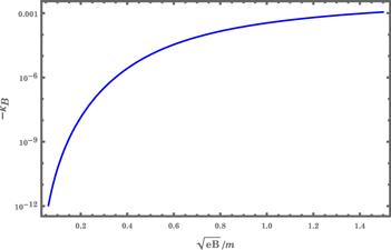
Figure 3. The magnetic correction to the AMM of electron/muon as a function of the dimensionless quantity $\sqrt{{eB}}/m$, with m = me or mμ. |
As addressed in the introduction, the AMM of a quark plays a vital role for QCD matter under a strong magnetic field when the magnitude of the magnetic field becomes comparable with the quark mass square, such as in the early evolution of cosmological phase transition [43], non-central heavy ion collisions [12], and neutron-star merger [44]. The exact value of the AMM of quarks under a magnetic field remains unknown because of its nonperturbative nature. In most literature, the AMM of quarks under a magnetic field was taken as a positive constant. We can extend the magnetic field-dependent AMM of electrons to the case of quarks and investigate its effect on the magnetized QCD matter. We will report the results in the forthcoming work [42].