


Abbreviations
$u$ Displacement variable
$t$ Independent variable
$\alpha $ Fractal dimension
$S$ Fractal parameter
$\eta ,\,\mu $ The first and second coefficients of damping
$Q$ The coefficient of Duffing
$f(u)$ Restoring force
$F(u;\alpha )$ Equivalent restoring force
${\eta }_{eq}(\alpha ),\,{\mu }_{eq}(\alpha )$ Equivalent coefficients
${\omega }_{0}$ Linear frequency
${\rm{\Omega }}$ Non-conservative frequency
$\omega $ Conservative frequency
1. Introduction
Many different phenomena in physics and the engineering sciences are represented by nonlinear systems of differential equations, which include the third-order derivative. The importance of these phenomena appears greatly in many applications in daily life, for example, in electrical circuits, mechanics, dynamic processes, and acoustics [1–6]. The study of this type of system has gained importance since Schot defined the rate of change of the acceleration vector as the jerk (1978) [7]. The investigation of the acceleration of charged particles that emit radiation is one of the most important applications for the time-jerk equation in the field of laser physics. As common, the influences of studying surface tension may be represented by an equation that has third order. Therefore, studying the flow control of the boundary layer of viscous liquid which has a free surface is also a critically important application of this equation in the field of surface tension. Furthermore, in the human body examination, the study of the physiological balance clarifies a significant application for the Duffing-jerk equation in the field of biology [8] and [9].
One can consider the nonlinear oscillation phenomenon as a significant phenomenon in engineering, biology, and physics, which can be described by oscillator equations such as Duffing oscillators [10]. To deal with these nonlinear oscillators, several numerical and analytical approaches have been applied. For this type of system, analytical periodic solutions must be obtained, so Nayfeh and Mook [11] and Nayfeh [12] introduced the classical perturbation and multiple-scale method to analyze Duffing oscillator with damping force, respectively. The homotopy perturbation approach was also proposed by He [13–15]. Recently, El-Dib has used the non-perturbative technique to introduce a simple approach for solving nonlinear jerk-Duffing and Rayleigh–Helmholtz–Duffing equations in [16–18]. Ji-Huan He, a famous Chinese mathematician, has recently proposed 'He's frequency formulation’ [19], an easy formula for determining the frequency of nonlinear models. One of the most significant benefits of this procedure over other perturbation techniques is its high accuracy and simplicity of use when dealing with nonlinear systems, particularly non-conservative models [20]. Several scientists were extremely motivated to use this methodology for this reason to demonstrate its scientific accuracy. For more recent applications of He's frequency formulation, Ma [21] suggested an alternative modification for He's frequency formulation to solve a quintic/cubic Duffing equation. For modeling a damped forced parametric pendulum model, Alyousef et al [22] used He's frequency formulation. Feng and Niu [23] also estimated a new analytical solution for a fractal Toda model. For an electromechanical system on a nano-scale, He et al [24] have extended He's frequency formula for faster calculation of the pull voltage. Also, an efficient simulation of He's formula has recently been published by El-Dib and his group [25–29].
The fractal studying is an interesting idea that has distinctive applications in assorted areas, for instance, the physical phenomena of the hierarchical structure, diffusion, thermal conductivity within branched networks, meteorology, fluids flow resistance in micro-channels, ocean and atmosphere dynamics, nuclear and petroleum engineering, thermo elasticity, and materials design [30–38]. As a result of these important applications, the study of fractals was a fertile field for many scientists. Sheng et al [39] studied the fractal model of shale through a porous medium. For the fluid flow through a porous structure, another fractal model was investigated by Miao et al [40]. Further, by utilizing the mechanism of homotopy perturbation, He et al [41] evaluated an approximate solution for the Toda oscillator with fractal space. By employing the Hamilton principle, He et al [42.] also introduced a modern fractal modification to calculate a periodic solution for a fractal Duffing oscillator. During the steady state, an exact solution of a damped forced fractal oscillator was calculated in [43]. Furthermore, by applying two-scale fractal derivatives, Feng [44] obtained an analytic solution for Duffing oscillator in fractal space. Ain and He [45] investigated the two-scale dimension to investigate some applications of fractal theory. Anjum and his colleagues [46, 47] also introduced the two-scale fractal theory to investigate the mathematical models of tsunami waves and population, respectively. By using the two-scale fractal calculus, He and El-Dib [48] analyzed the application of the fractal Shabat–Zhiber model. The fractal with two-scale and harmonic balance techniques was also applied by Lu and Chen [49] to analyze a fractal Yao-Cheng oscillator. Further, Ain et al [50] used the two-scale fractal dimension to provide an in-depth study of the alcohol-drinking model that includes the fractional derivative. Zuo and Liu [51] investigated a fractal rheological problem for SiC pastes using a fractal derivative. A two-scale technique was also used by Ain et al [52] and Yang et al [53] to investigate time-fractional heat transport and Varicella-Zoster virus models, respectively. Also, based on the two-scale fractal calculus, Huang et al [54]. developed a permeability fractal model for a porous medium. Moreover, Wang [55] used He's frequency formula to solve another nonlinear fractal oscillator. In [56, 57], the same author also proposed a clear frequency formulation to investigate the nonlinear oscillators with fractal space. In addition, Tian [58] introduced another frequency formulation to deal with a system of fractal oscillators. Lately, in [59], He et al also employed fractals with two-scale derivatives to investigate a fractal vibration. In the field of microgravity space, Wang [60] also used the Fourier series to propose a new technique for a class of fractal nonlinear oscillators that have discontinuities. For more analysis of the dynamical systems, El-Nabulsi et al [61] achieved a novel local derivative operator with fractal via both Hamiltonian and Lagrangian functions. On the other hand, there are a lot of effective contributions to ‘analytical approximation’ and ‘fractional/fractal’ modeling in the literature. By employing natural transforms and fractional calculus, respectively, Nadeem et al [62] and Elgazery [63] proposed numerical and analytical solutions to the fractional nonlinear Newell-Whitehead-Siegel model. A numerical solution of a reaction-diffusion/advection model with time fraction derivatives in porous media was also introduced by Pandey et al [64]. El-Dib et al [65] also provided an analytical solution for the Klein–Gordon model with time fraction derivatives. For more recent and significant contributions, see [28, 66–68].
Furthermore, the usage of nonlinear fractal vibrations has spread significantly in the literature over the past few decades due to its great role in studying practical problems for several disciplines of science and engineering that cannot be solved by traditional techniques. Consequently, fractal oscillation behaves differently than traditional behavior since there are important applications for the Duffing-Jerk equation in our everyday activities as mentioned in the literature. Recently, El-Dib and Elgazery [66, 67] have suggested an efficient novel approach to convert the fractal model into a traditional one. Hence, the current study aims to extend El-Dib and Elgazery's studies to introduce a novel technique to solve a fractal damping Duffing-jerk oscillator. This article is constructed in such a way that the details of the basic idea to convert the fractal space to a smooth one are presented in section 2 . The methodology and solution are described in section 3 . The stability analysis is outlined in section 4 . The numerical illustrations are displayed in section 5 . Finally, in section 6 the conclusions are given.
2. The basic idea is to transform from fractal space to smooth space
When the fractal dimension is positive or zero integers, the two-scale fractional derivative is consistent with the nth-order differential derivatives [48].
The fractal derivative via He's definition is written as follows [59, 68–71]:
$\begin{eqnarray}\displaystyle \frac{{{\rm{d}}}^{\alpha }u}{{\rm{d}}{t}^{\alpha }}={\rm{\Gamma }}(1+\alpha )\mathop{{\rm{L}}{\rm{i}}{\rm{m}}}\limits_{\begin{array}{l}t-{t}_{0}\to {\rm{\Delta }}t\\ \,{\rm{\Delta }}t\ne 0\end{array}}\displaystyle \frac{u(t)-u({t}_{0})}{{(t-{t}_{0})}^{\alpha }}\,,\,\end{eqnarray}$
here along the $t$ direction, $\alpha $ is the fractal dimension. Additionally, this fractal derivative exhibits some of the following characteristics [25, 41, 69, 72]: $\begin{eqnarray}\mathop{{\rm{L}}{\rm{i}}{\rm{m}}}\limits_{\alpha \to 0}\displaystyle \frac{{\rm{d}}u}{{\rm{d}}{t}^{\alpha }}=u\,,\,\mathop{{\rm{L}}{\rm{i}}{\rm{m}}}\limits_{\alpha \to 1}\displaystyle \frac{{\rm{d}}u}{{\rm{d}}{t}^{\alpha }}\,=\dot{u}\, \ {\rm{and}}\,\ \mathop{{\rm{L}}{\rm{i}}{\rm{m}}}\limits_{\alpha \to 2}\displaystyle \frac{{\rm{d}}u}{{\rm{d}}{t}^{\alpha }}\,=\ddot{u},\end{eqnarray}$
here the traditional derivative concerning the variable $t$ is mentioned with the over dots.As evidenced by the literature, the traditional approach of substituting ${t}^{\alpha }$ with $\tau $ cannot produce the desired result. Except in exceptional instances, the solution cannot be readily available. At this point, it is urgently necessary to investigate a novel strategy that enables discovering the damping fractal model solution. It is necessary to convert the fractal model into its continuous space equivalent. A good strategy is to adhere to El-Dib and Elgazery's most recent publications [66, 67]. The following proposal is offered to address this property:
$\begin{eqnarray}\displaystyle \frac{{\rm{d}}u}{{\rm{d}}{t}^{\alpha }}={S}^{\alpha }\,\cos \left(\tfrac{1}{2}\pi \alpha \right)\,u+{S}^{\alpha -1}\,\sin \left(\tfrac{1}{2}\pi \alpha \right)\,\dot{u};\,0\lt \alpha \lt 1.\end{eqnarray}$
This is called the global He's a fractal derivative of first-order which represents a modification to He's fractal derivative. Consequently, it can be verified that the nth global fractal derivative has the form $\begin{eqnarray}\begin{array}{c}\displaystyle \frac{{\rm{d}}u}{{\rm{d}}{t}^{n\alpha }}={\left({S}^{\alpha }\cos \left(\tfrac{1}{2}\pi \alpha \right)+{S}^{\alpha -1}\sin \left(\tfrac{1}{2}\pi \alpha \right){\rm{D}}\right)}^{n}u;\\ n=1,2,\mathrm{3...}\end{array}\end{eqnarray}$
where the operator ${\rm{D}}$ refers to the first classical derivative with respect to the variable $t.$Over the past few decades, the use of nonlinear fractal vibrations has grown dramatically due to its important role in researching real-world issues in many engineering and science disciplines that cannot be solved by conventional methods. Fractal oscillation performs differently from conventional behavior as a result. Consider a fractal system of the Duffing-jerk oscillating which has numerous significant applications in daily life in the form
$\begin{eqnarray}\begin{array}{l}\displaystyle \frac{{\rm{d}}u}{{\rm{d}}{t}^{3\alpha }}+\eta \displaystyle \frac{{\rm{d}}u}{{\rm{d}}{t}^{2\alpha }}+\mu \displaystyle \frac{{\rm{d}}u}{{\rm{d}}{t}^{\alpha }}+f(u)=0;\\ \,0\lt \alpha \lt 1;\,u(0)=A,\displaystyle \frac{{\rm{d}}}{{\rm{d}}{t}^{\alpha }}u(0)=0,\displaystyle \frac{{\rm{d}}}{{\rm{d}}{t}^{2\alpha }}u(0)=0,\end{array}\end{eqnarray}$
here $u,$ $\displaystyle \frac{{\rm{d}}u}{{\rm{d}}{t}^{3\alpha }},$ $\displaystyle \frac{{\rm{d}}u}{{\rm{d}}{t}^{2\alpha }},$ and $\displaystyle \frac{{\rm{d}}u}{{\rm{d}}{t}^{\alpha }}$ are a dynamical variable, third-, second- and third-order time fractal derivatives, respectively. The definition of restoring force $f(u)$ can take the form $\begin{eqnarray}f(u)={\omega }_{0}u+Q{u}^{3}.\end{eqnarray}$
This system in the case of $\alpha =1$ the form [1] $\begin{eqnarray}\dddot{u}+\eta \ddot{u}+\mu \dot{u}+{\omega }_{0}u+Q{u}^{3}=0,\end{eqnarray}$
where the first, second, and third derivatives of t are indicated by the upper dots. Here $\eta ,$ $\mu ,$ and $Q$ are constants and ${\omega }_{0}$ is a constant natural frequency.The original fractal system (5 ) can be converted to the traditional form by letting $n=1$ one time, $n=2$ a second time, and finally $n=3$ into He's global fractal derivative (4 ); and employing the results into (5 ) gives
$\begin{eqnarray}\begin{array}{l}{b}^{3}(\alpha ){\left({\rm{D}}+a(\alpha )\right)}^{3}u+\eta {b}^{2}(\alpha ){\left({\rm{D}}+a(\alpha )\right)}^{2}u\\ \,+\mu b(\alpha )\left({\rm{D}}+a(\alpha )\right)u+{\omega }_{0}u+Q{u}^{3}=0,\end{array}\end{eqnarray}$
where the notations $a(\alpha )$ and $b(\alpha )$ are $\begin{eqnarray}a(\alpha )=S\,\cot \left(\tfrac{1}{2}\pi \alpha \right),\,{\rm{and}}\,b(\alpha )={S}^{\alpha -1}\,\sin \left(\tfrac{1}{2}\pi \alpha \right).\end{eqnarray}$
Equation (8 ) is the critically damped Duffing-jerk oscillator, in the continuous space, in which the form is3 ), can be accomplished through the comparison between the original restoring force $f(u)$ and the equivalent restoring force $F(u;\alpha ).$ The comparison between the nonlinearity in $u$ leads to ${b}^{3}(\alpha )\to 1.$ This occurs only when $\alpha \to 1;$ otherwise, ${b}^{3}(\alpha )\ne 1\,$ in which case the critical result may be obtained from the comparison of the original linear stiffness with the equivalent linear stiffness. This yields the following value of the fractal parameter $S:$ 15 ) has been plotted for $S$ as a function $\alpha .$ The system considered in this calculation is for $\eta =2$ and $\mu =3$ with some variation in ${\omega }_{0}$ (${\omega }_{0}=0.1,\,0.2,\,0.3,\,0.4$). The calculations appear in figure 1. It is observed that $S$ and $\alpha $ have a nonlinear relationship where $S$ increases as $\alpha $ increases till a maximum point then the parameter $S$ has gradually decreased. Also, the curve of the parameter $S$ has been affected by increasing the parameter ${\omega }_{0}.$ In figure 2, the parameter $S$ is drawn versus ${\omega }_{0}$ the variation in $\alpha .$ It is noted that as ${\omega }_{0}$ increases, the parameter $S$ increases. Two roles are observed for the parameter $\alpha $ growth. The right end for the $S$-curve has moved up as $\alpha $ increases from $\alpha =0$ to $0.7,$ then, as the value of $\alpha $ continues to increase until $\alpha \leqslant 1,$ the right end of the $S$-curve has moved in the direction of decreasing $S.$ This is the interpretation of the nonlinear relationship between the parameters $S$ and $\alpha .$
$\begin{eqnarray}\dddot{u}+{\eta }_{eq}(\alpha )\ddot{u}+{\mu }_{eq}\,(\alpha )\dot{u}+F(u,\alpha )=0,\end{eqnarray}$
here the coefficients ${\eta }_{eq}(\alpha ),\,{\mu }_{eq}(\alpha )$ and the restoring force $F(u,\alpha )$ are given by $\begin{eqnarray}{\eta }_{eq}(\alpha )=3a(\alpha )+\displaystyle \frac{\eta }{b(\alpha )},\end{eqnarray}$
$\begin{eqnarray}{\mu }_{eq}(\alpha )=3{a}^{2}(\alpha )+2\eta \displaystyle \frac{a(\alpha )}{b(\alpha )}+\displaystyle \frac{\mu }{{b}^{2}(\alpha )},\end{eqnarray}$
$\begin{eqnarray}\begin{array}{l}F(u;\alpha )=\left({a}^{3}(\alpha )+\eta \displaystyle \frac{{a}^{2}(\alpha )}{b(\alpha )}+\mu \displaystyle \frac{a(\alpha )}{{b}^{2}(\alpha )}+\displaystyle \frac{{\omega }_{0}}{{b}^{3}(\alpha )}\right)u \,+\displaystyle \frac{Q{u}^{3}}{{b}^{3}(\alpha )}.\end{array}\end{eqnarray}$
As a result, the initial conditions in the smooth space are changed to have amplitude–displacement oscillations and are only allowed to have initial acceleration and velocity that are not equal to zero as: $\begin{eqnarray}u(0)=A,\,\dot{u}(0)=-A\,a\left(\alpha \right),\,\ddot{u}(0)=A\,{a}^{2}\left(\alpha \right).\end{eqnarray}$
The estimation of the fractal parameter $S,$ which first appears in the transformation ( $\begin{eqnarray}\begin{array}{l}{S}^{3} =\displaystyle \frac{{\omega }_{0}{S}^{3\alpha }{\sin }^{3}\left(\tfrac{1}{2}\pi \alpha \right)}{{S}^{3\alpha }{\cos }^{3}\left(\tfrac{1}{2}\pi \alpha \right)+\eta {S}^{2\alpha }{\cos }^{2}\left(\tfrac{1}{2}\pi \alpha \right)+\mu {S}^{\alpha }\,\cos \left(\tfrac{1}{2}\pi \alpha \right)+{\omega }_{0}}.\end{array}\end{eqnarray}$
It is noted that in the limiting case as $\alpha \to 0,$ the parameter $S$ should be zero, which is true. On the other side, in the limiting case when $\alpha \to 1,$ the abovementioned relationship will be satisfied automatically. To explain the connection between the two parameters $S$ $\alpha ,$ the relation (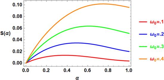
Figure 1. Representation of the fractal parameter $S$ versus the parameter $\alpha $ for variation of ${\omega }_{0}.$ |
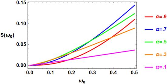
Figure 2. Representation of the fractal parameter $S$ as a function of the linear frequency ${\omega }_{0}$ with the variation of $\alpha .$ |
3. The methodology and solution
To convert the nonlinear equation (10 ) into the equivalent linearized form, the following trial solution may be introduced:16 ), the equivalent linearized form of (10 ) may be sought as:16 ) into (18 ) the final integration gives
$\begin{eqnarray}U(t)=A-\displaystyle \frac{A}{{\rm{\Omega }}}\,a\left(\alpha \right)\sin \,{\rm{\Omega }}t+\displaystyle \frac{A}{{{\rm{\Omega }}}^{2}}{a}^{2}\left(\alpha \right)\left(1-\,\cos \,{\rm{\Omega }}t\right),\end{eqnarray}$
where ${\rm{\Omega }}$ is the non-conservative frequency to be determined later. Because of ( $\begin{eqnarray}\dddot{u}+{\eta }_{eq}(\alpha )\ddot{u}+{\mu }_{eq}\,(\alpha )\dot{u}+\omega \left({\rm{\Omega }}\right)u=0,\end{eqnarray}$
where the conservative frequency $\omega \left({\rm{\Omega }}\right)$ is estimated [26], in the presence of the damping forces, as $\begin{eqnarray}\omega \left({\rm{\Omega }}\right)=\displaystyle \frac{\displaystyle {\int }_{0}^{T}UF(U){\rm{d}}t}{\displaystyle {\int }_{0}^{T}{U}^{2}{\rm{d}}t};\,T=\displaystyle \frac{2\pi }{{\rm{\Omega }}},\end{eqnarray}$
Employing ( $\begin{eqnarray}\begin{array}{l}\omega \left({\rm{\Omega }}\right)=\displaystyle \frac{a}{{b}^{2}}\left({a}^{2}{b}^{2}+ab\eta +\mu \right)+\displaystyle \frac{1}{{b}^{3}}{\omega }_{0}\\ +\displaystyle \frac{\left({a}^{2}+{{\rm{\Omega }}}^{2}\right)\left(35{a}^{4}+40{a}^{2}{{\rm{\Omega }}}^{2}+8{{\rm{\Omega }}}^{4}\right)}{4{{\rm{\Omega }}}^{4}{b}^{3}\left(3{a}^{2}+2{{\rm{\Omega }}}^{2}\right)}{A}^{2}Q.\end{array}\end{eqnarray}$
Equation (17 ) is a linear critically damped jerk oscillator with constant coefficients depending on the fractional parameter $\alpha .$ The following method is used to get the exact solution for equation (17 ). Let us assume a solution in the following manner.17 ). Employing (20 ) into equation (17 ) gives21 ) can be performed as:14 ).
$\begin{eqnarray}u(t)=\xi (t){{\rm{e}}}^{\phi \,t}.\end{eqnarray}$
It is understood that three significant unknown parameters, the total damping rate coefficient $\phi ,$ unknown function $\xi (t),$ and non-conservative frequency ${\rm{\Omega }}$ are needed for covering the conservative frequency $\omega $ in the equivalent equation ( $\begin{eqnarray}\dddot{\xi }\left(t\right)+\displaystyle \frac{1}{2}P^{\prime\prime} \left(\phi \right)\ddot{\xi }\left(t\right)+P^{\prime} \left(\phi \right)\dot{\xi }\left(t\right)+\left(P\left(\phi \right)+\omega \right)\xi \left(t\right)=0,\end{eqnarray}$
where the derivative for $\phi $ is represented by the dash, and $P\left(\phi \right)$ is estimated to be $\begin{eqnarray}P\left(\phi \right)={\phi }^{3}+{\eta }_{eq}\left(\alpha \right){\phi }^{2}+{\mu }_{eq}\left(\alpha \right)\phi .\end{eqnarray}$
The velocillator configuration requires that the unknown parameter $\phi $ has to fulfill the ensuing equation: $\begin{eqnarray}{\phi }^{3}+{\eta }_{eq}\left(\alpha \right){\phi }^{2}+{\mu }_{eq}\left(\alpha \right)\phi +\omega \left({\rm{\Omega }}\right)=0.\end{eqnarray}$
Keeping in mind the above condition, the solution of equation ( $\begin{eqnarray}\xi \left(t\right)=\int {{\rm{e}}}^{-\frac{1}{2}\left(3\varphi +{\eta }_{eq}\right)t}\left({C}_{1}\,\cos \,{\rm{\Omega }}t+{C}_{2}\,\sin \,{\rm{\Omega }}t\right)\,{\rm{d}}t+{C}_{3},\end{eqnarray}$
where the arbitrary constants ${C}_{i};i=1,2,3$ are established by the equivalent initial conditions (Making the above integration and applying conditions (14 ) yield solution (20 ) as:22 ) into (26 ) reduces it to23 ) and inserting the real root into (27 ) gives the desired real values of ${{\rm{\Omega }}}^{2}.$
$\begin{eqnarray}\begin{array}{l}u\left(t\right)=\frac{A(a+\phi ){{\rm{e}}}^{-\displaystyle \frac{1}{2}\left(\phi +{\eta }_{eq}\right)t}}{{\rm{\Omega }}\left(4{\Omega }^{2}+9{\phi }^{2}+6\phi {\eta }_{eq}+{\eta }_{eq}^{2}\right)}\\ \left[4{\rm{\Omega }}\left(2\phi +{\eta }_{eq}-a\right)\cos \,{\rm{\Omega }}t\right.\\ \left.+\left(-4{\Omega }^{2}+3{\phi }^{2}-6a\phi +{\eta }_{eq}\left({\eta }_{eq}+4\phi -2a\right)\right)\sin \,{\rm{\Omega }}t\right]\\ +\frac{A{e}^{\phi t}\left[4{\Omega }^{2}+{\eta }_{eq}\left({\eta }_{eq}+2\phi -4a\right)+{\left(2a-\phi \right)}^{2}\right]}{\left(4{\Omega }^{2}+9{\phi }^{2}+6\phi {\eta }_{eq}+{\eta }_{eq}^{2}\right)}.\end{array}\end{eqnarray}$
It is noted that the frequency ${\rm{\Omega }},$ established due to the velocillator technology, is given by $\begin{eqnarray}{{\rm{\Omega }}}^{2}=P^{\prime} \left(\phi \right)-\displaystyle \frac{1}{16}{P^{\prime\prime} }^{2}\left(\phi \right).\end{eqnarray}$
Employing ( $\begin{eqnarray}{{\rm{\Omega }}}^{2}=\displaystyle \frac{1}{4}\left(3{\phi }^{2}+2{\eta }_{eq}\phi +4{\mu }_{eq}-{\eta }_{eq}^{2}\right).\end{eqnarray}$
This is the frequency formula as a function of the damping rate coefficient $\phi .$ Solving the cubic equation (4. Stability analysis
There is an effective condition making the obtained solution (25 ) bounded. That is, ${{\rm{\Omega }}}^{2}$ must have positive values, which requires that the polynomial of $\phi $ in (27 ) must be positive. Since this polynomial is of the second-degree in $\phi ,$ then the stability requires that the discernment must be negative which leads to23 ), the following procedure can be utilized:
$\begin{eqnarray}4{\mu }_{eq}-{\eta }_{eq}^{2}\gt 0.\end{eqnarray}$
As seen, the frequency ${{\rm{\Omega }}}^{2}$ has been sought in terms of the parameter $\phi .$ To reformulate it in terms of the coefficients of the linearized equation (To perform the frequency equation (27 ) free of the parameter $\phi ,$ condition (23 ) can be used for this purpose. The procedure depends on removing ${\phi }^{2}$ and ${\phi }^{3}$ from (23 ); and using (27 ) yields the following relationship:29 ) into (27 ), finally the following formula for the frequency ${\rm{\Omega }}$ is estimated explicitly as
$\begin{eqnarray}\phi =-\displaystyle \frac{9\omega +{\eta }_{eq}^{3}+4{\eta }_{eq}\left({{\rm{\Omega }}}^{2}-{\mu }_{eq}\right)}{12{{\rm{\Omega }}}^{2}+{\eta }_{eq}^{2}-3{\mu }_{eq}}.\end{eqnarray}$
Employing ( $\begin{eqnarray}\begin{array}{l}{{\rm{\Omega }}}^{6}-\displaystyle \frac{1}{2}\left(3{\mu }_{eq}-{\eta }_{eq}^{2}\right){{\rm{\Omega }}}^{4}+\displaystyle \frac{1}{16}{\left({\eta }_{eq}^{2}-3{\mu }_{eq}\right)}^{2}{{\rm{\Omega }}}^{2}\\ -\displaystyle \frac{1}{64}\left[27{\omega }^{2}+\displaystyle \frac{1}{2}{\eta }_{eq}\left(2{\eta }_{eq}^{2}-9{\mu }_{eq}\right)\omega -{\mu }_{eq}^{2}\left({\eta }_{eq}^{2}-4{\mu }_{eq}\right)\right]\\ =\,0.\end{array}\end{eqnarray}$
To numerically explain the stability behavior, the root ${{\rm{\Omega }}}^{2}$ of equation (30 ) has been plotted versus the fractal parameter $\alpha $ for some variation of the linear frequency ${\omega }_{0}.$ The computations are done assuming that the system has $A=1,\,Q=0.1,\,\eta =2,$ and $\mu =3.$ In the case where $\alpha =1,$ this system is chosen to satisfy the stability condition (28 ). The frequency curve has divided the plane $\left({{\rm{\Omega }}}^{2}-\alpha \right)$ into two regions. This curve separates the positive side from the negative side. The region characterized with positive values represents the stable region, while the other side refers to the unstable region. The results are displayed in figure 5. Inspecting this graph, two roles are observed. The first role conserves the variation of the fractional parameter $\alpha .$ It is shown that the increase $\alpha $ leads to an increase in the unstable region. The maximum instability occurs corresponding to the largest value of $\alpha \lt 1.$ This means that the decrease in $\alpha $ has a stabilizing influence. This behavior is consistent with what is observed in figures 3 and 4. The second important observation concerns the variation of the original linear frequency ${\omega }_{0}.$ It has been shown that the increase in ${\omega }_{0}$ causes the transition curve to move in the direction of increasing ${{\rm{\Omega }}}^{2},$ leaving more increase in the unstable area. This behavior demonstrates the destabilizing effects of increasing ${\omega }_{0}.$
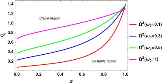
Figure 3. Demonstrated a stability diagram for the influence of the parameter $\alpha $ on the fractal solution ( |
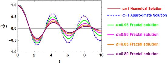
Figure 4. The representation of the solution ( |
5. Numerical illustration
For the same system taken into consideration in figure 3, the numerical representation of the solution (25 ) has been produced using two distinct values of the linear frequency ${\omega }_{0}.$ The numerical calculations are displayed in figures 4 and 5. Figure 4 represents the system having ${\omega }_{0}=1.75.$ The analytical solution (25 ) and the numerical solution of equation (7 ), applied in the instance of $\alpha =1,$ are compared. This graph analysis reveals a damping behavior with a highly good matching between the numerical and analytical representation. For checking the impact of $\alpha $ on the profile of the analytical solution (25 ), the calculations, with the variation in the fractal parameter $0\lt \alpha \lt 1,$ are done and collected in this graph, too. It is noted that the amplitude of the vibration decreases as $\alpha $ decreases. This means that the dwindling in the value of $\alpha $ has backed up the system-dampening behavior. This simulates the stability behavior as shown in figure 3.
Investigating the same system in figure 4, except that ${\omega }_{0}=2,$ is the subject of figure 5. A significant change in the numerical and analytical solution behavior is observed as ${\omega }_{0}$ increases. There is a divergence in the amplitude of the vibration as $t$ increases. The major observation in this examination is that the decrease in $\alpha $ hinders the developmental role of the amplitude of oscillation and transforms it into a damping behavior. This is a great advantage of the fractal parameter effect. Finally, it is evident from the preceding figures that fractal oscillation behaves differently from traditional behavior. Therefore, there is a great advantage to studying the fractal model and the influence of the fractal parameter, which has important contributions to the analysis of dynamic oscillation.

Figure 5. The representation of the solution ( |
6. Conclusion
Fractal oscillation performs differently from conventional behavior, so in the current work, a new analysis of the fractal-damping Duffing-jerk oscillator has been proposed. Two converting approaches have been applied in this investigation. The first one concerns the transforming of the fractal derivative to the traditional one to describe the fractal Duffing jerk oscillator into continuous space. The procedure is an insightful and comprehensive formularization based on a global definition of the He's fractal derivative. So the limitations of this new analysis are the restrictions of the He's definition. The second involves turning a nonlinear jerk oscillator into a damping linear jerk oscillator using a non-perturbative methodology. This alternative form of the fractal jerk appears with equivalent coefficients having contributions of the fractal order $\alpha .$ The analytical solution of the linear jerk oscillation is given and the stability behavior is briefly explained. To illustrate the operability and effectiveness of the method, the analytical solution, with $\alpha $ very closer to unity, is compared with the numerical one, which shows a great agreement. The contribution of the fractal derivative order $\alpha $ has an impact on the jerk stability profile. The effectiveness of the fractal derivative order $\alpha $ has been explained graphically, which shows that the decrease in its values plays a destabilizing influence. Further, it can transform the behavior of the growth in the oscillation amplitude into the behavior of damping in the amplitude of the vibration characteristics.
Acknowledgments
The authors express their gratitude to Princess Nourah bint Abdulrahman University Researchers Supporting Project number (PNURSP2023R17), Princess Nourah bint Abdulrahman University, Riyadh, Saudi Arabia.
Competing interests and funding
The authors got no financial support for this article, publication, or authorship of the current investigation.
Statements and declarations
In connection with the publication of this search, the authors declare that there are no competing interests.