


1. Introduction
So far, most experimental results have demonstrated the success of the Standard Model (SM). However, the theoretical difficulties of the theory itself have led people to believe that the SM is merely an effective theory, with the expectation of new physics (NP) potentially emerging at higher energy scales [1]. Due to the lack of clear signs of new physics, the SM effective field theory (SMEFT) [2–5] has become a popular theoretical tool for studying experimental results in a model-independent way. In most cases, NP effects are expected to manifest in physical processes that are described by dimension-6 operators of SMEFT. However, in some special cases, the contribution of dimension-8 operators may be more important [6–11]. These cases include anomalous quartic gauge coupling (aQGC) and neutral triple gauge coupling (nTGC), which have been the subject of many theoretical studies and experimental measurements [12–42]. These couplings are fixed by electroweak gauge bosons only. Another type of anomalous gauge coupling that does not exist in the SM is the quartic coupling between gluons and electroweak (EW) vector bosons. They can be described by dimension-8 operators, which are operators contributing to gluonic quartic gauge couplings (gQGCs) [7]. The quartic couplings of gluons to EW gauge bosons arise in the Born–Infeld (BI) extension of the SM, which was originally proposed to set an upper limit on the strength of the electromagnetic field [6]. It has been shown that the BI also appears in the theories inspired by M theory [43–45]. Recently, the gQGCs have been studied at the Large Hadron Collider (LHC)[7, 46].
High-energy collisions can directly generate new particles, while precise measurements assist us in identifying the indirect effects of unknown new physics and understanding the dynamics of known particles. The muon collider capitalizes on the advantages of two strategic approaches to exploit the complementarity between energy and precision. The inception of concepts pertaining to muon colliders dates back to earlier time [47–51]. At present, the energy frontier attainable by muon colliders remains undetermined. Ongoing investigations are centered on a 10 TeV configuration, with a targeted integrated luminosity of 10 ab−1 [52, 53]. With the high energy and high luminosity, the muon collider not only possesses a stronger capability for probing NP compared to the LHC but also has the ability for more precise measures. As a result, high-energy muon colliders have gained much attention in the community [38–41, 54–64]. The muon colliders are ideal places to study the dimension-8 operators, including those contributing to the gQGCs. In a high-energy muon collider, the initial state muons emit low-virtuality vector bosons. The weak-boson fusion process transforms the muon collider into a high-luminosity vector boson collider [52, 65]. The gQGCs can affect the process ${\mu }^{+}{\mu }^{-}\to {jj}\nu \bar{\nu }$ via both the vector boson fusion (VBF) processes and the tri-boson productions. In this paper, we study the sensitivity of the process ${\mu }^{+}{\mu }^{-}\to {jj}\nu \bar{\nu }$ to the gQGCs.
The rest of this paper is organized as follows. In section 2 , the dimension-8 operators contributing to gQGCs are introduced. In section 3 , we compare the VBF process with the tri-boson process and discuss the unitarity bound on the operator coefficients. We also present our event selection strategy at muon colliders with different energies and luminosities. The numerical results of the constraints on the coefficients are presented in section 4 . In section 5 , we summarize and draw our conclusions.
2. Dimension-8 gluonic QGC operators
Although there are many possibilities for new physics at higher energy scales above the EW one, the low energy effective field theory (EFT) should be subject to the SM SU(3)c × SU(2)L × U(1)Y gauge symmetries. A convenient way to take these symmetries into account is the SMEFT [66], which includes systematically all the allowed interactions with mass dimension d > 4. The extra dimensions are compensated by inverse powers of a mass scale M that is associated with heavy new particles. The gQGCs appear at dimension-8 level with 1/M4 suppression [7],
$\begin{eqnarray}{O}_{{gT},0}\equiv \displaystyle \frac{1}{16{M}_{0}^{4}}\displaystyle \sum _{a}{G}_{\mu \nu }^{a}{G}^{a,\mu \nu }\times \displaystyle \sum _{i}{W}_{\alpha \beta }^{i}{W}^{i,\alpha \beta },\end{eqnarray}$
$\begin{eqnarray}{O}_{{gT},1}\equiv \displaystyle \frac{1}{16{M}_{1}^{4}}\displaystyle \sum _{a}{G}_{\alpha \nu }^{a}{G}^{a,\mu \beta }\times \displaystyle \sum _{i}{W}_{\mu \beta }^{i}{W}^{i,\alpha \nu },\end{eqnarray}$
$\begin{eqnarray}{O}_{{gT},2}\equiv \displaystyle \frac{1}{16{M}_{2}^{4}}\displaystyle \sum _{a}{G}_{\alpha \mu }^{a}{G}^{a,\mu \beta }\times \displaystyle \sum _{i}{W}_{\nu \beta }^{i}{W}^{i,\alpha \nu },\end{eqnarray}$
$\begin{eqnarray}{O}_{{gT},3}\equiv \displaystyle \frac{1}{16{M}_{3}^{4}}\displaystyle \sum _{a}{G}_{\alpha \mu }^{a}{G}_{\beta \nu }^{a}\times \displaystyle \sum _{i}{W}^{i,\mu \beta }{W}^{i,\nu \alpha },\end{eqnarray}$
$\begin{eqnarray}{O}_{{gT},4}\equiv \displaystyle \frac{1}{16{M}_{4}^{4}}\displaystyle \sum _{a}{G}_{\mu \nu }^{a}{G}^{a,\mu \nu }\times {B}_{\alpha \beta }{B}^{\alpha \beta },\end{eqnarray}$
$\begin{eqnarray}{O}_{{gT},5}\equiv \displaystyle \frac{1}{16{M}_{5}^{4}}\displaystyle \sum _{a}{G}_{\alpha \nu }^{a}{G}^{a,\mu \beta }\times {B}_{\mu \beta }{B}^{\alpha \nu },\end{eqnarray}$
$\begin{eqnarray}{O}_{{gT},6}\equiv \displaystyle \frac{1}{16{M}_{6}^{4}}\displaystyle \sum _{a}{G}_{\alpha \mu }^{a}{G}^{a,\mu \beta }\times {B}_{\nu \beta }{B}^{\alpha \nu },\end{eqnarray}$
$\begin{eqnarray}{O}_{{gT},7}\equiv \displaystyle \frac{1}{16{M}_{7}^{4}}\displaystyle \sum _{a}{G}_{\alpha \mu }^{a}{G}_{\beta \nu }^{a}\times {B}^{\mu \beta }{B}^{\nu \alpha },\end{eqnarray}$
where ${G}_{\mu \nu }^{a}$ is gluon field strengths, ${W}_{\mu \nu }^{i}$ and Bμν are electroweak field strengths. Since gluons carry QCD color, denoted by the a superscript of ${G}_{\mu \nu }^{a}$, the gQGC operators must contain an even number of gluon field strengths, such as ${G}_{\mu \nu }^{a}{G}^{a,\alpha \beta }$, so as to be colorless. The same thing applies for the SU(2)L × U(1)Y gauge boson field strengths, for example ${W}_{\mu \nu }^{i}{W}^{i,\alpha \beta }$ and BμνBαβ. Another symmetry to be imposed is Lorentz invariance. There are four different Lorentz-invariant contractions, as shown above. Hence we must consider eight gQGC operators in total.The total and differential cross-sections are largely determined by the Lorentz structure of the gQGC operators. The eight operators can be classified into four pairs {OgT,(0,4), OgT,(1,5), OgT,(2,6), OgT,(3,7)}, each with a same Lorentz structure.
The hierarchical structure of the cross-sections generated by the eight gQGC operators is manifest in the 95% C.L. lower bounds derived from the ATLAS data [7] are
$\begin{eqnarray}\begin{array}{rcl}{M}_{0} & \geqslant & 1040\,\mathrm{GeV},\,{M}_{1}\geqslant 777\,\mathrm{GeV},\\ {M}_{2} & \geqslant & 750\,\mathrm{GeV},\,{M}_{3}\geqslant 709\,\mathrm{GeV},\\ {M}_{4} & \geqslant & 1399\,\mathrm{GeV},\,{M}_{5}\geqslant 1046\,\mathrm{GeV},\\ {M}_{6} & \geqslant & 1010\,\mathrm{GeV},\,{M}_{7}\geqslant 954\,\mathrm{GeV}.\end{array}\end{eqnarray}$
3. Features of the signal
3.1. Compare of the tri-boson process and the VBF process
The gQGCs can contribute to the process ${\mu }^{+}{\mu }^{-}\to {jj}\nu \bar{\nu }$ via both the VBF and tri-boson processes, the Feynman diagrams are shown in figure 1. When a new particle X presents in the final states, the relative scaling between the VBF and annihilation contribution is [67]
$\begin{eqnarray}\displaystyle \frac{{\sigma }_{\mathrm{VBF}}^{\mathrm{NP}}}{{\sigma }_{\mathrm{ann}}^{\mathrm{NP}}}\propto {\alpha }_{W}^{2}\displaystyle \frac{s}{{m}_{X}^{2}}{\mathrm{log}}^{2}\left(\displaystyle \frac{s}{{M}_{V}^{2}}\right)\mathrm{log}\left(\displaystyle \frac{s}{{M}_{X}^{2}}\right)\end{eqnarray}$
where ${\sigma }_{\mathrm{VBF}}^{\mathrm{NP}}$ and ${\sigma }_{\mathrm{ann}}^{\mathrm{NP}}$ are cross-sections of VBF and annihilation processes, respectively. MX,V denotes the masses of the X particle and the SM vector bosons, respectively. At high energies, the VBF process is double-logarithmic enhanced. However, it has been pointed out that, at lower energies the tri-boson process can be more sensitive to the dimension-8 operators [40]. Therefore, it is necessary to compare the contribution of tri-boson and VBF for the case of gQGCs.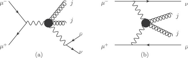
Figure 1. The Feynman diagrams of the gQGC contributions. The tri-boson contribution is shown in the left panel, while the VBF contribution is shown in the right panel. |
In the following, we consider the gQGC contribution to the process ${\mu }^{+}{\mu }^{-}\to \nu \bar{\nu }{gg}$. For simplicity, defining ${f}_{i}\equiv 1/16{M}_{i}^{4}$, the triboson and the VBF contributions (denoting as σtri and σVBF) at the leading order of ${M}_{Z,W}^{2}/s$ and at tree level are,4 ) and (5 ), the interference between σtri and σVBF are ignored. The σVBF is obtained using the effective vector boson approximation [68–70],
$\begin{eqnarray}\begin{array}{l}{\sigma }_{\mathrm{tri}}=\mathrm{Br}(Z\to \nu \bar{\nu })\times \displaystyle \frac{{e}^{2}{s}^{3}}{8847360{\pi }^{3}{c}_{W}^{2}{s}_{W}^{2}}\\ \quad \times \left\{{c}_{W}^{4}\left[24{f}_{0}^{2}+4{f}_{3}({f}_{0}+3{f}_{1}+{f}_{2})+8{f}_{0}{f}_{1}\right.\right.\\ \quad \left.\left.+12{f}_{0}{f}_{2}+14{f}_{1}^{2}+8{f}_{1}{f}_{2}+3{f}_{2}^{2}+4{f}_{3}^{2}\right]\right.\\ \quad \left.-2{c}_{W}^{2}{s}_{W}^{2}\left[2{f}_{7}({f}_{0}+3{f}_{1}+{f}_{2}+2{f}_{3})+24{f}_{0}{f}_{4}+4{f}_{0}{f}_{5}\right.\right.\\ \quad \left.\left.+6{f}_{0}{f}_{6}+4{f}_{1}{f}_{4}+14{f}_{1}{f}_{5}+4{f}_{1}{f}_{6}\right.\right.\\ \quad \left.\left.+6{f}_{2}{f}_{4}+4{f}_{2}{f}_{5}+3{f}_{2}{f}_{6}+2{f}_{3}{f}_{4}+6{f}_{3}{f}_{5}+2{f}_{3}{f}_{6}\right]\right.\\ \quad \left.+5{s}_{W}^{4}\left[24{f}_{4}^{2}+4{f}_{7}({f}_{4}+3{f}_{5}+{f}_{6})+8{f}_{4}{f}_{5}+12{f}_{4}{f}_{6}\right.\right.\\ \quad \left.\left.+14{f}_{5}^{2}+8{f}_{5}{f}_{6}+3{f}_{6}^{2}+4{f}_{7}^{2}\right]\right\}\end{array}\end{eqnarray}$
and $\begin{eqnarray}\begin{array}{l}{\sigma }_{\mathrm{VBF}}=\displaystyle \frac{{e}^{4}{s}^{3}}{4246732800000{\pi }^{5}{s}_{W}^{4}}\\ \quad \times \left\{600{\mathrm{log}}^{2}\left(\displaystyle \frac{s}{16{M}_{W}^{2}}\right)\left[800\left((6{f}_{0}^{2}+{f}_{0}(2{f}_{1}+3{f}_{2}+{f}_{3})\right)\right.\right.\\ \quad +1492{f}_{1}^{2}+52{f}_{1}(31{f}_{2}+21{f}_{3})+603{f}_{2}^{2}\\ \quad \left.+806{f}_{2}{f}_{3}+473{f}_{3}^{2}\right]\\ \quad -40\mathrm{log}\left(\displaystyle \frac{s}{16{M}_{W}^{2}}\right)\\ \quad \left[160800{f}_{0}^{2}+26800{f}_{0}(2{f}_{1}+3{f}_{2}+{f}_{3})\right.\\ \quad \left.+33944{f}_{1}^{2}+4{f}_{1}(9491{f}_{2}+5136{f}_{3})\right.\\ \quad \left.+16191{f}_{2}^{2}+18982{f}_{2}{f}_{3}+11836{f}_{3}^{2}\right]\\ \quad \left.+4526400{f}_{0}^{2}+754400{f}_{0}(2{f}_{1}+3{f}_{2}+{f}_{3})+764788{f}_{1}^{2}\right.\\ \quad \left.+877948{f}_{1}{f}_{2}+387588{f}_{1}{f}_{3}\right.\\ \quad \left.+408087{f}_{2}^{2}+438974{f}_{2}{f}_{3}+285497{f}_{3}^{2}\right\}\end{array}\end{eqnarray}$
where $\sqrt{s}$ is the c.m. energies of the muon colliders ${s}_{W}=\sin ({\theta }_{W})$ and ${c}_{W}=\cos ({\theta }_{W})$ with the weak mixing angle denoted as θW, $\mathrm{Br}(Z\to \nu \bar{\nu })$ is taken as 20%. In equations ( $\begin{eqnarray}\begin{array}{l}{\sigma }_{\mathrm{VBF}}({\mu }^{+}{\mu }^{-}\to \bar{\nu }\nu {gg})\\ \quad =\displaystyle \sum _{{\lambda }_{1}{\lambda }_{2}{\lambda }_{3}{\lambda }_{4}}\int {\rm{d}}{\xi }_{1}\\ \quad \times \int {\rm{d}}{\xi }_{2}{f}_{{{\rm{W}}}_{{\lambda }_{1}}^{-}/{\mu }^{-}}({\xi }_{1}){f}_{{{\rm{W}}}_{{\lambda }_{2}}^{+}/{\mu }^{+}}({\xi }_{2}){\sigma }_{{{\rm{W}}}_{{\lambda }_{1}}^{+}{{\rm{W}}}_{{\lambda }_{2}}^{-}\to \mathrm{gg}}(\hat{{\rm{s}}}),\\ {f}_{{W}_{+1}^{-}/{\mu }_{L}^{-}}(\xi )={f}_{{W}_{-1}^{+}/{\mu }_{L}^{+}}(\xi )=\displaystyle \frac{{e}^{2}}{8{\pi }^{2}{s}_{W}^{2}}\displaystyle \frac{{\left(1-\xi \right)}^{2}}{2\xi }\mathrm{log}\displaystyle \frac{{\mu }_{f}^{2}}{{M}_{W}},\\ {f}_{{W}_{-1}^{-}/{\mu }_{L}^{-}}(\xi )={f}_{{W}_{+1}^{+}/{\mu }_{L}^{+}}(\xi )=\displaystyle \frac{{e}^{2}}{8{\pi }^{2}{s}_{W}^{2}}\displaystyle \frac{1}{2\xi }\mathrm{log}\displaystyle \frac{{\mu }_{f}^{2}}{{M}_{W}},\\ {f}_{{W}_{0}^{-}/{\mu }_{L}^{-}}(\xi )={f}_{{W}_{0}^{+}/{\mu }_{L}^{+}}(\xi )=\displaystyle \frac{{e}^{2}}{8{\pi }^{2}{s}_{W}^{2}}\displaystyle \frac{1-\xi }{\xi },\\ {f}_{{W}_{\lambda }^{\pm }/{\mu }_{R}^{\pm }}=0,\,\,\,\,{f}_{{W}_{\lambda }^{\pm }/{\mu }^{\pm }}=\displaystyle \frac{{f}_{{W}_{\lambda }^{\pm }/{\mu }_{L}^{\pm }}+{f}_{{W}_{\lambda }^{\pm }/{\mu }_{R}^{\pm }}}{2},\end{array}\end{eqnarray}$
where $\sqrt{\hat{s}}=\sqrt{{\xi }_{1}{\xi }_{2}s}$ is the c.m. energy of W+W− → gg, and μf is the factorization scale set to be $\sqrt{\hat{s}}/4$ [70].The numerical results of equations (4 ) and (5 ) are shown in figure 2. The detector simulation is not included until the Monte Carlo (MC) simulation is applied. It can be seen that the tri-boson contribution is larger than the VBF at about $\sqrt{s}\lt 5\,\mathrm{TeV}$, at $\sqrt{s}=30\,\mathrm{TeV}$, σVBF is about 5 times of σtri. Therefore the contribution of tri-boson is not negligible. In this paper, σVBF, σtri, and the interference between them are considered as the signal of the gQGCs.

Figure 2. σtri in equation ( |
Apart from that, note that OgT,4,5,6,7 operators do not contribute to the W-boson fusion processes. Since the energies considered are mainly above 5 TeV, in this paper, we only consider the contributions of the OgT,0,1,2,3 operators. However, we shall emphasise that the process WW → gg provides a chance to study the OgT,0,1,2,3 operators separately, compared with the pp → γγ and pp → Zγ processes where the contributions from OgT,i and OgT,i+4 are proportional to each other [46].
3.2. Unitarity bound
The SMEFT is not UV completed. As an EFT, the SMEFT is only valid under a certain energy scale. One of the signals when the SMEFT is no longer valid is the violation of unitarity. With dimension-8 operators, the amplitude of the process W+W− → gg grows as ${\hat{s}}^{2}$ which leads to the violation of unitarity [71–73] at large enough energy. The partial wave unitarity bound [74–76] is often used to check whether the energy scale considered is already invalid. For the subprocess ${W}_{{\lambda }_{1}}^{+}{W}_{{\lambda }_{2}}^{-}\to {g}_{{\lambda }_{3}}{g}_{{\lambda }_{4}}$, where λi correspond to the helicities, the amplitude can be expanded as [77]
$\begin{eqnarray}\begin{array}{l}{ \mathcal M }({W}_{{\lambda }_{1}}^{+}{W}_{{\lambda }_{2}}^{-}\to {g}_{{\lambda }_{3}}{g}_{{\lambda }_{4}})\\ \quad =\,8\pi \displaystyle \sum _{J}\left(2J+1\right)\sqrt{1+{\delta }_{{\lambda }_{3},{\lambda }_{4}}}{e}^{{\rm{i}}(\lambda -\lambda ^{\prime} )\varphi }{{d}}_{\lambda \lambda ^{\prime} }^{{\rm{J}}}(\theta ){{T}}^{J}\end{array}\end{eqnarray}$
where λ = λ1 − λ2, $\lambda ^{\prime} ={\lambda }_{3}-{\lambda }_{4}$, θ and φ are zenith and azimuth angles of the one of the gluons in the final state, respectively, and ${d}_{\lambda \lambda ^{\prime} }^{J}(\theta )$ are Wigner d-functions [77]. The partial wave unitarity bound is ∣TJ∣ ≤ 2 [74] which is widely used in previous works [33, 35–39, 78–81].At leading order of $\hat{s}$, the relevant helicity amplitudes are8 ), and therefore are not presented for simplicity. Assuming one operator at a time, the tightest bounds are
$\begin{eqnarray}\begin{array}{l}{ \mathcal M }({W}_{+}^{+}{W}_{+}^{-}\to {g}_{+}{g}_{+})=\displaystyle \frac{{\hat{s}}^{2}}{16}(4{f}_{0}+{f}_{2}+{f}_{3}),\\ { \mathcal M }({W}_{+}^{+}{W}_{+}^{-}\to {g}_{-}{g}_{-})\\ =\,\displaystyle \frac{{\hat{s}}^{2}}{64}\left(16{f}_{0}+(2{f}_{1}+{f}_{3})\cos (2\theta )+6{f}_{1}+4{f}_{2}-{f}_{3}\right),\\ { \mathcal M }({W}_{+}^{+}{W}_{-}^{-}\to {g}_{+}{g}_{-})=\displaystyle \frac{{\hat{s}}^{2}}{16}{e}^{2{\rm{i}}\phi }{\cos }^{4}\left(\displaystyle \frac{\theta }{2}\right)(2{f}_{1}+{f}_{2}+{f}_{3}).\\ \end{array}\end{eqnarray}$
There are other helicity amplitudes which lead to same unitarity bounds as those derived from equation ( $\begin{eqnarray}\displaystyle \frac{{\hat{s}}^{2}| {f}_{0}| }{32\sqrt{2}\pi }\lt 2,\,\,\,\displaystyle \frac{{\hat{s}}^{2}| {f}_{1}| }{96\sqrt{2}\pi }\lt 2,\,\,\,\displaystyle \frac{{\hat{s}}^{2}| {f}_{\mathrm{2,3}}| }{128\sqrt{2}\pi }\lt 2.\end{eqnarray}$
Table 1. The upper bounds of coefficients ∣fi∣ and lower bounds of Mi in the sense of partial wave unitarity at different energies. |
| $\sqrt{\hat{s}}(\mathrm{TeV})$ | 3 | 10 | 14 | 30 |
| ∣f0∣(TeV−4) | 3.5 | 0.028 | 0.0074 | 0.00035 |
| M0(GeV) | 365.56 | 1222.31 | 1704.76 | 3655.55 |
| ∣f1∣(TeV−4) | 10.5 | 0.085 | 0.022 | 0.001 |
| M1(GeV) | 277.76 | 926.01 | 1298.27 | 2811.71 |
| ∣f2,3∣(TeV−4) | 14.0 | 0.114 | 0.030 | 0.004 |
| M2,3(GeV) | 258.49 | 860.49 | 1201.41 | 1988.18 |
3.3. Event selection strategy
The background in this study is the SM contribution to ${\mu }^{+}{\mu }^{-}\to {jj}\nu \bar{\nu }$. The process μ+μ− → jj is suppressed by the s-channel propagator, and can be further suppressed by the cuts on the missing energy, therefore is ignored. The process ${\mu }^{+}{\mu }^{-}\to {jj}\nu \nu \bar{\nu }\bar{\nu }$ is suppressed by more EW couplings and therefore is also ignored.
The typical Feynman diagrams for the background at tree level are shown in figure 3. An important feature is that the two jets are both from quarks, which is different from the case of gQGCs where the two jets are both from the gluons. As a consequence, there is no interference term between the SM and the gQGCs. Once the efficiencies of the event selection strategy for both the background and the signal are obtained, the cross-section can be read out.
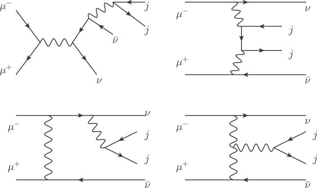
Figure 3. Typical Feynman diagrams of the SM contribution. |
To investigate the event selection strategy, the MC simulation is carried out with the help of the MadGraph5_aMC@NLO [82, 83] toolkit including a parton shower using Pythia82 [84]. The standard cuts are used as the default. The parton distribution function is NNPDF2.3 [85]. A fast detector simulation is then applied using Delphes [86] with the muon collider card. In the event generation, the complete syntax ${\mu }^{+}{\mu }^{-}\to {jj}{\nu }_{l}{\bar{\nu }}_{l}$ is used, and the standard cuts are set as the default of ‘MadGraph5_aMC@NLO', the relevant cuts for jets are transverse momentum ${p}_{T}^{j}\gt 20\,\mathrm{GeV}$ and pseudo-rapidity ηj < 5.0, and ΔRjj > 0.4, where ${\rm{\Delta }}R=\sqrt{{\rm{\Delta }}{\phi }_{{jj}}^{2}+{\rm{\Delta }}{\eta }_{{jj}}^{2}}$ and where Δφjj and Δηjj are the difference between the azimuth angles and pseudo-rapidities of any two jets.
At the energies of the muon colliders, the SM cross-sections (denoted as σSM) are obtained and listed in table 2. In the SM, the cross-section grows slowly with the energy.
Table 2. The cross-sections of the SM contribution and the upper bounds of coefficients ∣fi∣ used in the phenomenological study. The cross-sections of the gQGCs are also shown. |
| $\sqrt{s}(\mathrm{TeV})$ | 3 | 10 | 14 | 30 |
| σSM(pb) | 0.8688 | 1.4548 | 1.6087 | 1.8988 |
| ∣f0∣(TeV−4) | 1 | 0.012 | 0.004 | 0.00035 |
| σgT,0(pb) | 0.00321 | 0.00115 | 0.00112 | 0.00114 |
| ∣f1∣(TeV−4) | 1.5 | 0.02 | 0.007 | 0.0006 |
| σgT,1(pb) | 0.00355 | 0.00138 | 0.00144 | 0.00134 |
| ∣f2,3∣(TeV−4) | 3 | 0.03 | 0.012 | 0.0012 |
| σgT,2(pb) | 0.00383 | 0.000956 | 0.00134 | 0.00178 |
| σgT,3(pb) | 0.00412 | 0.000924 | 0.00127 | 0.00161 |
The signal events are generated by assuming one operator at a time. The sensitivity of the process ${\mu }^{+}{\mu }^{-}\to {jj}\nu \bar{\nu }$ to the gQGCs can be estimated with respect to the significance defined as [87, 88]4 ) and (5 ). The coefficients are chosen so that the signal significance of the VBF contributions are about Sstat = 2 ∼ 3 before cuts at luminosity L = 1 ab−1, L = 10 ab−1 for $\sqrt{s}=3\,\mathrm{TeV}$ and $\sqrt{s}\geqslant 10\,\mathrm{TeV}$, respectively [52, 53]. The coefficients at different energies are listed in table 2. Note that they are also chosen to be within the partial wave unitarity bounds in table 1. The contributions of the gQGCs (denoted as σgT,i) obtained by MC are also shown in table 2.
$\begin{eqnarray}{{ \mathcal S }}_{{\rm{stat}}}=\sqrt{2\left[({N}_{\mathrm{bg}}+{N}_{s})\mathrm{ln}(1+{N}_{s}/{N}_{\mathrm{bg}})-{N}_{s}\right]},\end{eqnarray}$
where Ns = NaQGC − NSM and Nbg = NSM. The Nbg can be obtained by σSM and the luminosities of the muon colliders, where the Ns can be provisionally estimated using σtri + σVBF where σtri and σVBF are given in equations (To investigate the kinematic features, we require that the final states contain at least two jets, which is denoted as the Nj cut. To suppress the events from the process μ+μ− → jj, we also require a minimal ${{/}\!\!\!\!\!{p}}_{T}$ for the events, where ${{/}\!\!\!\!\!{p}}_{T}$ is the transverse missing energy. ${{/}\!\!\!\!\!{p}}_{T}$ can also be used to suppress the events from the SM contribution to ${\mu }^{+}{\mu }^{-}\to {jj}\nu \bar{\nu }$. This is because the signal grows with the energy so that for the tri-boson signal events, the neutrinos are typically from a highly boosted Z boson. Since neutrinos play a role similar to that of the residual jets of the VBF processes at a hadron collider, similar to the standard VBF cut [89], the neutrinos are expected to be back-to-back. For the VBF signal events, although the neutrinos are back-to-back, the net transpose momentum is still typically larger than the case of the SM. The normalized distributions of ${{/}\!\!\!\!\!{p}}_{T}$ for the backgrounds and signals are shown in figure 4. We require the events to have a large ${{/}\!\!\!\!\!{p}}_{T}$, which is denoted as the ${{/}\!\!\!\!\!{p}}_{T}$ cut.
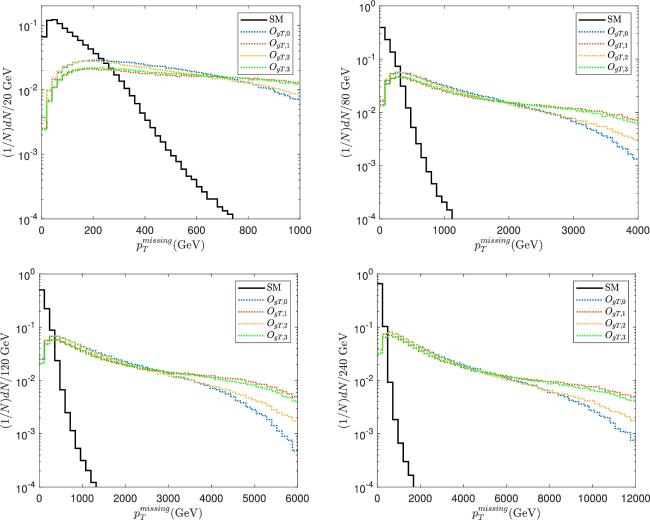
Figure 4. The normalized distributions of ${{/}\!\!\!\!\!{p}}_{T}$ for the SM and gQGCs at different energies. The top left panel corresponds to $\sqrt{s}=3\,\mathrm{TeV}$, the top right panel corresponds to $\sqrt{s}=10\,\mathrm{TeV}$, the bottom left panel corresponds to $\sqrt{s}=14\,\mathrm{TeV}$, and the bottom right panel corresponds to $\sqrt{s}=30\,\mathrm{TeV}$. |
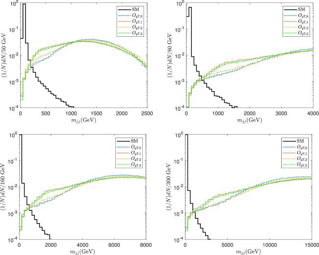
Due to the same reason, for both the tri-boson and VBF signal events, the jets are energetic. As a result, the invariant mass of the hardest two jets (denoted as mjj) should be large for the signal events. The normalized distributions of mjj for the background and signal are shown in figure 5. We require the events to have a large mjj, which is denoted as the mjj cut.
Figure 5. Same as figure 4 but for mjj. |
At different energies, we use different cuts. The event selection strategies are summarized in table 3. The cross-sections after cuts are listed in table 4. The efficiencies of the cuts (denoted as ε) are also shown in table 4. It can be seen that the event selection strategies can suppress the background significantly.
Table 3. The event selection strategies at different energies. |
| $\sqrt{s}$ | ${{/}\!\!\!\!\!{p}}_{T}$ | mjj |
|---|---|---|
| (TeV) | ||
| 3 | >50 GeV | >1 TeV |
| 10 | >100 GeV | >3 TeV |
| 14 | >100 GeV | >5 TeV |
| 30 | >200 GeV | >10 TeV |
Table 4. The contributions of the SM and gQGCs after cuts. The efficiencies of the cuts are shown in the last row. |
| $\sqrt{s}$ | cut | SM | OgT,0 | OgT,1 | OgT,2 | OgT,3 |
|---|---|---|---|---|---|---|
| (TeV) | (fb) | (fb) | (fb) | (fb) | (fb) | |
| Nj | 722.9 | 3.21 | 3.52 | 3.82 | 4.10 | |
| 3 | $\not{P}_T$ | 536.7 | 3.15 | 3.47 | 3.74 | 4.04 |
| mjj | 0.885 | 2.49 | 2.27 | 2.85 | 2.74 | |
| ε | 0.102% | 77.6% | 63.9% | 74.4% | 66.5% | |
| $\sqrt{s}$ | cut | SM | OgT,0 | OgT,1 | OgT,2 | OgT,3 |
| (TeV) | (fb) | (fb) | (fb) | (fb) | (fb) | |
| Nj | 1191.9 | 1.15 | 1.37 | 0.955 | 0.921 | |
| 10 | $\not{P}_T$ | 508.2 | 1.12 | 1.34 | 0.930 | 0.902 |
| mjj | 0.256 | 0.961 | 1.06 | 0.799 | 0.728 | |
| ε | 0.0176% | 83.6% | 76.8% | 83.6% | 78.8% | |
| $\sqrt{s}$ | cut | SM | OgT,0 | OgT,1 | OgT,2 | OgT,3 |
| (TeV) | (fb) | (fb) | (fb) | (fb) | (fb) | |
| Nj | 1315.5 | 1.12 | 1.43 | 1.34 | 1.26 | |
| 14 | $\not{P}_T$ | 531.9 | 1.10 | 1.42 | 1.31 | 1.24 |
| mjj | 0.105 | 0.846 | 1.02 | 1.03 | 0.916 | |
| ε | 0.00653% | 75.5% | 70.8% | 76.9% | 72.1% | |
| $\sqrt{s}$ | cut | SM | OgT,0 | OgT,1 | OgT,2 | OgT,3 |
| (TeV) | (fb) | (fb) | (fb) | (fb) | (fb) | |
| Nj | 1542.4 | 1.14 | 1.33 | 1.78 | 1.61 | |
| 30 | $\not{P}_T$ | 256.4 | 1.11 | 1.30 | 1.73 | 1.57 |
| mjj | 0.0532 | 0.914 | 1.04 | 1.46 | 1.27 | |
| ε | 0.00280% | 80.2% | 77.6% | 82.0% | 78.9% |
4. Constraints on the coefficients
Assuming one operator at a time, without the interference between the SM and the gQGCs, the cross-section after cuts can be expressed as,10 ). The integrated luminosities for both the ‘conservative' and ‘optimistic' cases are considered [52, 53]. As a result, we can obtain the projected sensitivities on fi and Mi by taking 2σ, 3σ or 5σ significance. The results are shown in tables 5 and 6. The expected constraints on f2 and f3 are close to each other, which is indicated by the fact that the leading helicity amplitudes for O2,3 are the same.
$\begin{eqnarray}\sigma ={\epsilon }_{\mathrm{SM}}{\sigma }_{\mathrm{SM}}+{\epsilon }_{{gT},i}\displaystyle \frac{{f}_{i}^{2}}{{\tilde{f}}_{i}^{2}}{\sigma }_{{gT},i}({\tilde{f}}_{i})\end{eqnarray}$
where σSM and ${\sigma }_{{gT},i}({\tilde{f}}_{i})$ are the cross-sections of the SM and the gQGCs at ${\tilde{f}}_{i}$, and εSM and εgT,i are the cut efficiencies of the SM and gQGC events, respectively. Taking ${\tilde{f}}_{i}$ as the ones in table 2, numerical results of σSM and σgT,i are listed in table 2, and εSM and εgT,i are listed in table 4. The expected constraints at muon colliders can be estimated by the signal significance defined in equation (Table 5. The projected sensitivities on the aQGC coefficients at the muon colliders with different c.m. energies and integrated luminosities for the ‘conservative' case. |
| ${{ \mathcal S }}_{{\rm{stat}}}$ | 3 TeV | 10 TeV | 14 TeV | 30 TeV | |
|---|---|---|---|---|---|
| 1 ab−1 | 10 ab−1 | 10 ab−1 | 10 ab−1 | ||
| 2 | <155 | <1.24 | <0.351 | <0.025 | |
| ∣f0∣ | 3 | <191 | <1.52 | <0.432 | <0.03 |
| (10−3TeV−4) | 5 | <248 | <1.96 | <0.561 | <0.04 |
| 2 | >0.796 | >2.67 | >3.65 | >7.07 | |
| M0 | 3 | >0.756 | >2.53 | >3.47 | >6.71 |
| (TeV) | 5 | >0.709 | >2.38 | >3.25 | >6.29 |
| 2 | <244 | <1.96 | <0.561 | <0.040 | |
| ∣f1∣ | 3 | <300 | <2.41 | <0.689 | <0.049 |
| (10−3TeV−4) | 5 | <389 | <3.11 | <0.893 | <0.064 |
| 2 | >0.711 | >2.38 | >3.25 | >6.28 | |
| M1 | 3 | >0.675 | >2.26 | >3.09 | >5.96 |
| (TeV) | 5 | >0.633 | >2.12 | >2.89 | >5.58 |
| 2 | <436 | <3.39 | <0.957 | <0.068 | |
| ∣f2∣ | 3 | <535 | <4.16 | <1.17 | <0.083 |
| (10−3TeV−4) | 5 | <695 | <5.38 | <1.52 | <0.109 |
| 2 | >0.615 | >2.07 | >2.84 | >5.07 | |
| M2 | 3 | >0.585 | >1.97 | >2.70 | >5.23 |
| (TeV) | 5 | >0.548 | >1.85 | >2.53 | >4.90 |
| 2 | <445 | <3.55 | <1.01 | <0.073 | |
| ∣f3∣ | 3 | <546 | <4.35 | <1.25 | <0.090 |
| (10−3TeV−4) | 5 | <709 | <5.64 | <1.62 | <0.116 |
| 2 | >0.612 | >2.05 | >2.80 | >5.41 | |
| M3 | 3 | >0.582 | >1.95 | >2.66 | >5.14 |
| (TeV) | 5 | >0.545 | >1.82 | >2.49 | >4.81 |
Table 6. The projected sensitivities on the aQGC coefficients at the muon colliders with different c.m. energies and integrated luminosities for the ‘optimistic' case. |
| ${{ \mathcal S }}_{{\rm{stat}}}$ | 14 TeV | 30 TeV | |
|---|---|---|---|
| 20 ab−1 | 90 ab−1 | ||
| 2 | <2.95 | <0.144 | |
| ∣f0∣ | 3 | <3.63 | <0.176 |
| (10−4TeV−4) | 5 | <4.70 | <0.228 |
| 2 | >3.81 | >8.12 | |
| M0 | 3 | >3.62 | >7.71 |
| (TeV) | 5 | >3.40 | >7.23 |
| 2 | <4.71 | <0.231 | |
| ∣f1∣ | 3 | <5.78 | <0.284 |
| (10−4TeV−4) | 5 | <7.49 | <0.367 |
| 2 | >3.39 | >7.21 | |
| M1 | 3 | >3.23 | >6.85 |
| (TeV) | 5 | >3.02 | >6.42 |
| 2 | <8.03 | <0.390 | |
| ∣f2∣ | 3 | <9, 86 | <0.479 |
| (10−4TeV−4) | 5 | <12.8 | <0.619 |
| 2 | >2.97 | >6.33 | |
| M2 | 3 | >2.82 | >6.01 |
| (TeV) | 5 | >2.65 | >5.64 |
| 2 | <8.52 | <0.419 | |
| ∣f3∣ | 3 | <10.5 | <0.513 |
| (10−4TeV−4) | 5 | <13.5 | <0.664 |
| 2 | >2.93 | >6.22 | |
| M3 | 3 | >2.78 | >5.91 |
| (TeV) | 5 | >2.61 | >5.54 |
Compared with the expected constraints from the LHC in equation (2 ), the muon collider at $\sqrt{s}\geqslant 10\,\mathrm{TeV}$ has tighter constraints. Since the operators contributing to the gQGCs are dimension-8, not surprisingly, higher energy muon colliders are more advantageous in detecting the gQGCs. Taking OgT,0 as an example, at $\sqrt{s}=3\,\mathrm{TeV}$, the sensitivity will exceed that of the LHC when the luminosity is about 70 ab−1. However, for the luminosities in the ‘optimistic' case, i.e., L = 1, 10, 20 and 90 ab−1 for $\sqrt{s}=3,10,14$ and 30 TeV, respectively, the 2σlower bounds on M0 is about 27% of the c.m. energies of the muon collider, which indicates that the constraint on M0 will exceed that of the LHC at a $\sqrt{s}=4\,\mathrm{TeV}$ muon collider. Meanwhile, in the same case, the 2σlower bounds on M1,2,3 are about 24%, 21% and 20 ∼ 21% of $\sqrt{s}$, which are consistent with equation (2 ) in order of sensitivity. The above result can also be compared with the case of future hadron colliders such as the HL-LHC. In Ref. [46], taking OgT,0 as an example, the 2σ constraint on M0 by the pp → γγ channel is about 15% of $\sqrt{s}$, and the combined (combined of pp → γγ, pp → ℓ+ℓ−γ, ${pp}\to \nu \bar{\nu }\gamma $ and ${pp}\to q\bar{q}\gamma $ channels) constraint on M0 is about 22% of $\sqrt{s}$. Thus, the sensitivities of the muon colliders to the gQGCs are competitive with future hadron colliders, and are even better at the same c.m. energies.
5. Summary
The muon colliders which are also called vector boson colliders are ideal places to study the quartic gauge couplings. In this paper, we investigate the capability of future muon colliders to detect the gQGC in the framework of SMEFT. The cross-sections of the process ${\mu }^{+}{\mu }^{-}\to {jj}\nu \bar{\nu }$ with gQGCs present are calculated.
The gQGCs can affect the process ${\mu }^{+}{\mu }^{-}\to {jj}\nu \bar{\nu }$ via both tri-boson and VBF contributions. The tri-boson contribution is larger than the VBF when $\sqrt{s}\lt 5\,\mathrm{TeV}$, and is about 1/5 of the VBF at $\sqrt{s}=30\,\mathrm{TeV}$. Besides, the VBF process can be affected by OgT,0,1,2,3. Therefore, we focus on OgT,0,1,2,3 in this paper.
With partial wave unitarity bounds considered, the event selection strategy as well as the expected constraints on the operator coefficients are studied using MC simulation. For the luminosities in the ‘optimistic' case, 2σ lower bounds on M0,1,2,3 are about 27%, 24%, 21% and 20 – 21% of the c.m. energies of the muon colliders, respectively. Our results indicate that the muon colliders with $\sqrt{s}\gt 4\,\mathrm{TeV}$ can be more sensitive to the gQGCs than the LHC.