


1. Introduction
The multi-component Bose–Einstein condensate (BEC) is an ideal platform for studying the dynamics of vector solitons due to the advantages of macroscopic visibility and tunable atomic interactions [1, 2]. Many different vector solitons have been obtained in multi-component coupled BEC systems, such as bright-bright solitons [3–6], bright-dark solitons [7–9], dark-bright solitons [10–14], dark-dark solitons [15–17], bright-bright-dark solitons [9, 18] and dark-dark-bright solitons [18]. These studies on solitons in multi-component BECs are usually based on the integrable systems, such as the Manakov model [19] with equal inter- and intra-species interactions, and the coupled model with spin-dependent interactions [20–22]. Furthermore, in the non-integrable systems, in which interaction strengths are unequal, some vector soliton solutions can be obtained theoretically [23–27]. All the above-mentioned solitons are mainly mass solitons, due to the fact that their total mass densities have localized profiles. Multi-component BECs can be considered as pseudo-spin systems with different spin values [28–30]. In such systems, a localized spin polarization (the magnetic soliton) was the focus of both theoretical [24, 25] and experimental [31, 32] studies, due to its advantages in investigating solitary waves in non-Manakov cases and observing pure spin currents. Very recently, a spin soliton for the spin-1/2 system has been studied. The spin soliton's total mass density is also uniform and a soliton profile is shown on the spin density [33]. The spin solitons can admit spin-balanced or spin-imbalanced density backgrounds, thus having potential in the study of spin currents. Particularly, this type of soliton exhibits different dynamics under the effect of external forces compared with well-known vector solitons for the integrable cases. Spin soliton solutions for the spin-1 system have also been discovered [34]. These solutions are obtained based on the vector soliton solutions for the integrable Manakov model, and thus there are many constraints on the nonlinearity coefficients. These constraints can be relaxed and the variational method can provide much more exact analytical soliton solutions for two-component models with different nonlinearity coefficients [26]. Although the dark-bright soliton solutions for the three-component model are reported in [26], we employ a decoupling method to obtain spin soliton solutions more directly. We expect to reduce the constraints by using these soliton solutions for non-integrable models and obtain more general spin solitons in spin-1 systems.
In this paper, we utilize the soliton solutions in [26] to reduce the constraints in [34], and therefore extend the existence region of spin soliton solutions in nonlinearity coefficient space. We also perform spectral stability analysis and numerical simulations, and show that the spin solitons that admit spectral stability with discrete spectra are stable, while those with continuous spectra are metastable against weak noise. The existence region of spin solitons further enriches the family of solitons in BECs and provides a reference for investigations on non-integrable phenomena and experiments.
The structure of this paper is as follows. In section 2 , we give six spin soliton solutions as well as their constraints on nonlinear interaction strengths, and we carefully depict their properties and differences. In section 3 , we calculate the Bogoliubov–de Gennes excitation spectra of these spin solitons and test their stability using numerical simulations. In section 4 , we investigate the collisions between two spin solitons. When the speed is much lower than the upper limit, the soliton exhibits shape oscillation and slight acceleration after the collision. Finally, in section 5 , we summarize and discuss the results.
2. Spin-1 Bose–Einstein condensate system and spin soliton solutions
Under the mean-field approximation, the dynamics of a quasi-one-dimensional 87Rb BEC can be described by the following coupled Gross–Pitaevskii equations [20–22]:
$\begin{eqnarray}\begin{array}{l}{\rm{i}}\displaystyle \frac{\partial {\psi }_{1}}{\partial t}=-\displaystyle \frac{1}{2}\displaystyle \frac{{\partial }^{2}{\psi }_{1}}{\partial {x}^{2}}-({g}_{11}| {\psi }_{1}{| }^{2}+{g}_{12}| {\psi }_{2}{| }^{2}+{g}_{13}| {\psi }_{3}{| }^{2}){\psi }_{1}\\ \quad +{g}_{s}(| {\psi }_{1}{| }^{2}+| {\psi }_{2}{| }^{2}-| {\psi }_{3}{| }^{2}){\psi }_{1}+{g}_{s}{\psi }_{2}^{2}{\psi }_{3}^{* }+{V}_{1}(x){\psi }_{1},\end{array}\end{eqnarray}$
$\begin{eqnarray}\begin{array}{l}{\rm{i}}\displaystyle \frac{\partial {\psi }_{2}}{\partial t}=-\displaystyle \frac{1}{2}\displaystyle \frac{{\partial }^{2}{\psi }_{2}}{\partial {x}^{2}}-({g}_{21}| {\psi }_{1}{| }^{2}+{g}_{22}| {\psi }_{2}{| }^{2}+{g}_{23}| {\psi }_{3}{| }^{2}){\psi }_{2}\\ \quad +{g}_{s}(| {\psi }_{1}{| }^{2}+| {\psi }_{3}{| }^{2}){\psi }_{2}+2{g}_{s}{\psi }_{1}{\psi }_{2}^{* }{\psi }_{3}+{V}_{2}(x){\psi }_{2},\end{array}\end{eqnarray}$
$\begin{eqnarray}\begin{array}{l}{\rm{i}}\displaystyle \frac{\partial {\psi }_{3}}{\partial t}=-\displaystyle \frac{1}{2}\displaystyle \frac{{\partial }^{2}{\psi }_{3}}{\partial {x}^{2}}-({g}_{31}| {\psi }_{1}{| }^{2}+{g}_{32}| {\psi }_{2}{| }^{2}+{g}_{33}| {\psi }_{3}{| }^{2}){\psi }_{3}\\ \quad +{g}_{s}(| {\psi }_{2}{| }^{2}+| {\psi }_{3}{| }^{2}-| {\psi }_{1}{| }^{2}){\psi }_{3}+{g}_{s}{\psi }_{2}^{2}{\psi }_{1}^{* }+{V}_{3}(x){\psi }_{3},\end{array}\end{eqnarray}$
where ψi (i = 1, 2, 3) represents the wave function of the ith component and the symbol ‘*' indicates the complex conjugate, x and t respectively represent the spatial coordinate and time evolution, and Vi(x) denotes the weak axial trapping potential. The coefficients gii (gij) are the intra- (inter-) species interaction strengths given by the s-wave scattering length. Since gs/∣gij∣ is very small for 87Rb [35, 36], the spin-dependent terms can be safely ignored.Besides, the weak trapping potentials can be set to Vi = 0(i = 1, 2, 3) and the coupled Gross–Pitaevskii equations are reduced to coupled nonlinear Schrödinger equations (NLSEs). If gij are all equal, the equations will become the well-known Manakov model [19], which is completely integrable and can be solved exactly by the Darboux transformation [37, 38], Hirota bilinear method [39] and inverse-scattering method [40]. The Manakov case was the focus of previous theoretical studies; therefore, many different vector solitons have been obtained [3–18]. The realization of Feshbach resonance techniques enables the manipulation of the scattering length between three hyperfine states of atoms. In this case, the model is no longer integrable and its exact solutions cannot be obtained by the above-mentioned methods analytically. Very recently, a decoupling method was suggested and exact soliton solutions for the spin-1/2 and spin-1 BECs were derived. These solitons are not mass solitons due to their uniform mass densities (∑∣ψi∣2=1 for simplicity), and this character enables the reduced three-component system to still be seen as a pseudo-spin system. In particular, the pseudo-spin densities ${F}_{z}={{\rm{\Psi }}}^{\dagger }{\hat{F}}_{z}{\rm{\Psi }}\,=| {\psi }_{1}{| }^{2}-| {\psi }_{3}{| }^{2}$4(4The spin density ${F}_{z}={{\rm{\Psi }}}^{\dagger }{\hat{F}}_{z}{\rm{\Psi }}=| {\psi }_{1}{| }^{2}-| {\psi }_{3}{| }^{2}$, where ${\rm{\Psi }}={\left({\psi }_{1}\,{\psi }_{2}\,{\psi }_{3}\right)}^{{\rm{T}}}$ and the symbol ‘†' denotes the conjugate transpose. The spin-1 matrices, ${\hat{F}}_{x}=\tfrac{1}{\sqrt{2}}\left(\begin{array}{c}0\quad 1\quad 0\\ 1\quad 0\quad 1\\ 0\quad 1\quad 0\end{array}\right)$, ${\hat{F}}_{y}=\tfrac{{\rm{i}}}{\sqrt{2}}\left(\begin{array}{c}0\quad -1\quad 0\\ 1\quad 0\quad -1\\ 0\quad 1\quad 0\end{array}\right)$, and ${\hat{F}}_{z}=\tfrac{1}{\sqrt{2}}\left(\begin{array}{c}1\quad 0\quad 0\\ 0\quad 0\quad 0\\ 0\quad 0\quad -1\end{array}\right)$.) (where ${\rm{\Psi }}={\left({\psi }_{1}\,{\psi }_{2}\,{\psi }_{3}\right)}^{T}$ and the symbol ‘†' denotes the conjugate transpose) have soliton profiles, and therefore these solitons are called spin solitons.
Three-component coupled NLSEs can be decoupled into a two-component model with one scalar NLSE. The previously reported spin solitons were obtained when the two-component model was integrable, for which the exact soliton solutions can be derived analytically [34]. Recent research indicates that the exact analytical soliton solutions can be obtained for the non-integrable model [26]. Based on this, we can extend the coefficient space for spin soliton solutions, since the constraints on nonlinearity coefficients can be greatly relaxed. Now, one can obtain exact spin soliton solutions as long as the nonlinearity coefficients satisfy G1 = g12 = g21 and G2 = g13 = g31 = g23 = g32. According to the restriction on the uniform total mass density, we find that g33 is uniquely determined by the other coefficients:
$\begin{eqnarray}{g}_{33}=\displaystyle \frac{2{G}_{2}{g}_{11}-4{G}_{1}{G}_{2}+{G}_{1}^{2}+2{G}_{2}{g}_{22}-{g}_{11}{g}_{22}}{{g}_{11}-2{G}_{1}+{g}_{22}}.\end{eqnarray}$
For the non-integrable two-component model, there are four types of exact analytical soliton solutions, namely, bright-bright solitons, bright-dark solitons, dark-bright solitons and dark-dark solitons. Each of them exist in two separated regions with different constraint conditions [26]. When we go back to the original three-component equations, six types of spin soliton solutions can be obtained and they also have two different parts in the coefficient space. There is no essential difference between the same type of solitons in the two parts, and they are labeled as cases ‘−1' and ‘−2' in figure 1. In the subsequent discussions, we will mainly focus on case-1 solitons. The distribution map for the six spin soliton solutions are shown in figure 1 according to different constraint conditions on nonlinearity coefficients.

Figure 1. The extended existence regions for six types of spin soliton solutions in the nonlinearity coefficient space. The origin corresponds to the integrable Manakov model. Cases ‘−1' and ‘−2' are distinguished by the black plane. The black, red, blue and light green surfaces represent F1 = F4, F2 = F4, F1 + F2 − 2F4 = 0 and ${\left({F}_{4}-{F}_{2}+{F}_{1}\right)}^{2}-{F}_{1}{F}_{2}\,=\,0$, respectively. The spin solitons cannot exist on any surface. |
It should be emphasized that the existence of spin solitons directly depends on the difference between the nonlinearity coefficients Fi (i = 1, 2, 3, 4) rather than themselves. Here, Fi is the difference between G2 and other nonlinearity coefficients, where F1 = G2 − g11, F2 = G2 − g22, F3 = G2 − g33 and F4 = G2 − G1. Hence, spin soliton solutions obviously differ from solitons for the integrable model. If Fi=0, the model becomes the Manakov model, and spin solitons cannot exist. Specifically, spin soliton solutions cannot exist on any surface in figure 1. We present the specific classification of spin solitons based on Fi in table 1. Next, we give the generalised six spin soliton solutions, and carefully analyze their characteristics and differences.
Table 1. Classification of spin solitons based on the difference between nonlinearity coefficients Fi. Condition 1 divides spin soliton solutions into two cases where this condition is opposite. In this paper we mainly discuss case-1 solitons when F1 > F4. If one takes F1 < F4, the soliton solutions for case-2 can be obtained. Different spin solitons are discussed in the main text and shown as sub-figures (a)–(f) in figure 2. The coefficients Fi correspond to the difference between the interaction strengths, F1 = G2 − g11, F2 = G2 − g22, F3 = G2 − g33 and F4 = G2 − G1. |
| Constraint conditions | Soliton type | |||
|---|---|---|---|---|
| Condition 1 | Condition 2 | Condition 3 | Condition 4 | |
| F1 > F4 | F2 > F4 | F1 + F2 − 2F4 > 0 | ${\left({F}_{4}-{F}_{2}+{F}_{1}\right)}^{2}-{F}_{1}{F}_{2}\gt 0$ | BBD-1(a) |
| ${\left({F}_{4}-{F}_{2}+{F}_{1}\right)}^{2}-{F}_{1}{F}_{2}\lt 0$ | DDB-1(d) | |||
| F2 < F4 | F1 + F2 − 2F4 > 0 | ${\left({F}_{4}-{F}_{2}+{F}_{1}\right)}^{2}-{F}_{1}{F}_{2}\gt 0$ | DBB-1(c) | |
| ${\left({F}_{4}-{F}_{2}+{F}_{1}\right)}^{2}-{F}_{1}{F}_{2}\lt 0$ | BDB-1(b) | |||
| F1 + F2 − 2F4 < 0 | ${\left({F}_{4}-{F}_{2}+{F}_{1}\right)}^{2}-{F}_{1}{F}_{2}\gt 0$ | DBD-1(f) | ||
| ${\left({F}_{4}-{F}_{2}+{F}_{1}\right)}^{2}-{F}_{1}{F}_{2}\lt 0$ | BDD-1(e) | |||
In general, the spin solitons can be classified based on the soliton structures in the three components. Firstly, we show spin soliton solutions with two bright soliton components and one dark soliton component, which are a bright–bright–dark spin soliton (BBD), a bright–dark–bright spin soliton (BDB) and a dark–bright–bright spin soliton (DBB). The BBD solution can be written as:
$\begin{eqnarray}\begin{array}{rcl}{\psi }_{1} & = & \sqrt{\displaystyle \frac{{F}_{2}-{F}_{4}}{{F}_{4}^{2}-{F}_{1}{F}_{2}}}{w}_{1}{\rm{sech}} [{w}_{1}(x-{vt})]\\ & & \times {{\rm{e}}}^{\tfrac{1}{2}{\rm{i}}[(2{G}_{2}-{v}^{2}+{w}_{1}^{2})t+2{vx}]},\end{array}\end{eqnarray}$
$\begin{eqnarray}\begin{array}{rcl}{\psi }_{2} & = & \sqrt{\displaystyle \frac{{F}_{1}-{F}_{4}}{{F}_{4}^{2}-{F}_{1}{F}_{2}}}{w}_{1}{\rm{sech}} [{w}_{1}(x-{vt})]\\ & & \times {{\rm{e}}}^{\tfrac{1}{2}{\rm{i}}[(2{G}_{2}-{v}^{2}+{w}_{1}^{2})t+2{vx}]},\end{array}\end{eqnarray}$
$\begin{eqnarray}{\psi }_{3}\,=\,\displaystyle \frac{1}{\sqrt{{F}_{3}}}\left\{v-{\rm{i}}{w}_{1}\tanh [{w}_{1}(x-{vt})]\right\}{{\rm{e}}}^{{\rm{i}}({G}_{2}-{F}_{3})t},\end{eqnarray}$
where v and ${w}_{1}=\sqrt{{F}_{3}-{v}^{2}}$ are the velocity and inverse width of the soliton. It can be seen that the velocity v must be less than $\sqrt{{F}_{3}}$, where F3 is the difference between intra-species and inter-species interaction strengths of the ψ3 component. This indicates that the spin soliton differs from the vector soliton for the Manakov model, for which the soliton's maximum speed depends on the nonlinear interaction strength. Since the total mass density is uniform for spin solitons, the width and amplitude of the bright soliton directly depend on its velocity, which is inconsistent with that of the vector solitons [3–18, 41–47]. As an example, the mass density and spin density profiles for a static BBD are shown in figure 2(a). One can find that the background of the spin density is −1, while the maximum spin density can be varied within the region (−1, 1] by changing v and Fi.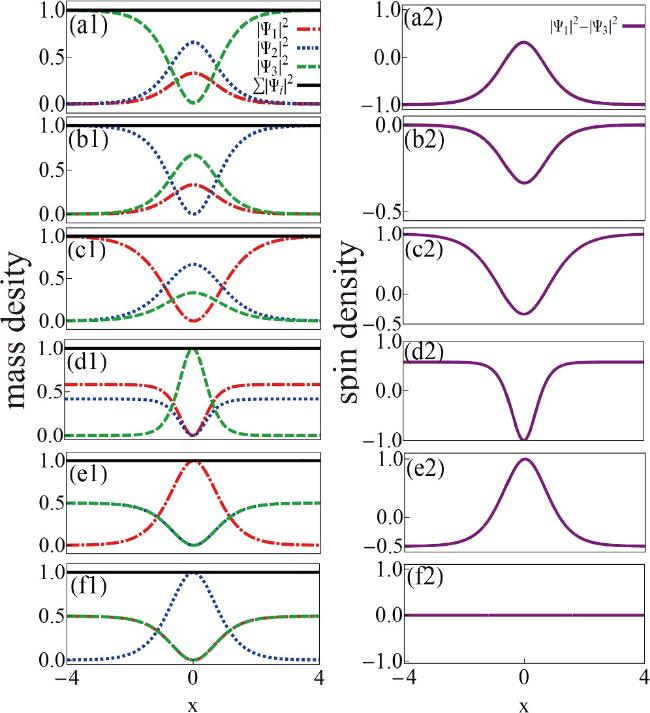
Figure 2. Mass and spin densities of six types of spin solitons: (a) BBD, (b) BDB, (c) DBB, (d) DDB, (e) BDD and (f) DBD. The red dash-dotted, blue dotted and green dashed lines represent three components, respectively. The total mass densities (black solid line) for all of these spin solitons are uniform. The parameters are: BBD:G1 = −3, G2 = −5, g11 = −6, g22 = −9/2. BDB: G1 = −3, G2 = −1, g11 = −4, g22 = −8/3. DBB: G1 = −7/2, G2 = −23/8, g11 = −4, g22 = −1. DBD: G1 = −2, G2 = −2, g11 = −4, g22 = −1. BDD: G1 = −3, G2 = −3, g11 = −2, g22 = −5. DDB: G1 = −5, G2 = −22/7, g11 = −7/2, g22 = −3. |
Next, the BDB solution is given as follows:
$\begin{eqnarray}\begin{array}{rcl}{\psi }_{1} & = & \sqrt{\displaystyle \frac{{F}_{2}-{F}_{4}}{{F}_{4}^{2}-{F}_{1}{F}_{2}}}{w}_{2}{\rm{sech}} [{w}_{2}(x-{vt})]\\ & & \times {{\rm{e}}}^{\tfrac{1}{2}{\rm{i}}[(2{G}_{1}-{v}^{2}+{w}_{2}^{2})t+2{vx}]},\end{array}\end{eqnarray}$
$\begin{eqnarray}{\psi }_{2}=\sqrt{\displaystyle \frac{{F}_{1}-{F}_{4}}{{F}_{1}{F}_{2}-{F}_{4}^{2}}}\left\{{\rm{i}}v+{w}_{2}\tanh \left[\left.{w}_{2}(x-{vt}\right)\right]\right\}{{\rm{e}}}^{{\rm{i}}({G}_{2}-{F}_{2})t},\end{eqnarray}$
$\begin{eqnarray}{\psi }_{3}=\sqrt{\displaystyle \frac{1}{-{F}_{3}}}{w}_{2}{\rm{sech}} [{w}_{2}(x-{vt})]{{\rm{e}}}^{\tfrac{1}{2}{\rm{i}}[(2{G}_{2}-{v}^{2}+{w}_{2}^{2})t+2{vx}]},\end{eqnarray}$
where ${w}_{2}=\sqrt{({F}_{1}{F}_{2}-{F}_{4}^{2})/({F}_{1}-{F}_{4})-{v}^{2}}$ is the inverse width of this type of spin soliton. It is easy to get a speed limit of $v\lt \sqrt{({F}_{1}{F}_{2}-{F}_{4}^{2})/({F}_{1}-{F}_{4})}$, which is evidently greater than that of BBD. In addition, BDB has a concave structure in the spin density distribution. Its spin density background is zero and the maximum spin density can be changed within (−1, 0], similar to the magnetic soliton [24, 25]. Figure 2(b) shows the mass density and spin density of a BDB with v = 0.The exact expression for DBB can be written as follows:
$\begin{eqnarray}{\psi }_{1}=\sqrt{\displaystyle \frac{{F}_{2}-{F}_{4}}{{F}_{1}{F}_{2}-{F}_{4}^{2}}}\left\{v-{\rm{i}}{w}_{3}\tanh [{w}_{3}(x-{vt})]\right\}{{\rm{e}}}^{{\rm{i}}({G}_{2}-{F}_{1})t},\end{eqnarray}$
$\begin{eqnarray}\begin{array}{rcl}{\psi }_{2} & = & \sqrt{\displaystyle \frac{{F}_{1}-{F}_{4}}{{F}_{4}^{2}-{F}_{1}{F}_{2}}}{w}_{3}{\rm{sech}} [{w}_{3}(x-{vt})]\\ & & \times {{\rm{e}}}^{\tfrac{1}{2}{\rm{i}}[(2{G}_{1}-{v}^{2}+{w}_{3}^{2})t+2{vx}]},\end{array}\end{eqnarray}$
$\begin{eqnarray}{\psi }_{3}\,=\,\displaystyle \frac{{w}_{3}}{\sqrt{-{F}_{3}}}{\rm{sech}} [{w}_{3}(x-{vt})]{{\rm{e}}}^{\tfrac{1}{2}{\rm{i}}[(2{G}_{2}-{v}^{2}+{w}_{3}^{2})t+2{vx}]},\end{eqnarray}$
where ${w}_{3}=\sqrt{({F}_{1}{F}_{2}-{F}_{4}^{2})/({F}_{2}-{F}_{4})-{v}^{2}}$. For DBB, the speed limit can be derived as $v\lt \sqrt{({F}_{1}{F}_{2}-{F}_{4}^{2})/({F}_{2}-{F}_{4})}$. As an example, we show one DBB with zero velocity in figure 2(c); its spin density shows a concave structure, where the background is 1 and the minimum spin density can be changed within [1, − 1). We emphasize that the above three types of spin solitons cannot be obtained by gauge transformations from each other, due to their different maximum speeds and spin distributions.When the spin soliton admits two dark soliton components together with one bright soliton component, another three types can be obtained. They are dark–dark–bright spin soliton (DDB), bright–dark–dark spin soliton (BDD) and dark–bright–dark spin soliton (DBD). The exact solution for DDB can be given as:
$\begin{eqnarray}{\psi }_{1}\,=\,\sqrt{\displaystyle \frac{{F}_{2}-{F}_{4}}{{F}_{1}{F}_{2}-{F}_{4}^{2}}}\left\{{\rm{i}}v+{w}_{4}\tanh [{w}_{4}(x-{vt})]\right\}{{\rm{e}}}^{{\rm{i}}({G}_{2}+{F}_{3})t},\end{eqnarray}$
$\begin{eqnarray}{\psi }_{2}\,=\,\sqrt{\displaystyle \frac{{F}_{1}-{F}_{4}}{{F}_{1}{F}_{2}-{F}_{4}^{2}}}\left\{{\rm{i}}v+{w}_{4}\tanh [{w}_{4}(x-{vt})]\right\}{{\rm{e}}}^{{\rm{i}}({G}_{2}+{F}_{3})t},\end{eqnarray}$
$\begin{eqnarray}{\psi }_{3}\,=\,\sqrt{1+\displaystyle \frac{{v}^{2}}{{F}_{3}}}{\rm{sech}} [{w}_{4}(x-{vt})]{{\rm{e}}}^{\tfrac{1}{2}{\rm{i}}[(2{G}_{2}-{v}^{2}+{w}_{4}^{2})t+2{vx}]},\end{eqnarray}$
where ${w}_{4}=\sqrt{-{F}_{3}-{v}^{2}}$, and the maximum speed for the DDB depends on the difference between the nonlinearity coefficients F3, namely, $v\lt \sqrt{-{F}_{3}}$. The mass density and spin density of a static DDB is shown in figure 2(d). Similarly, one can find that for the DDB, the spin density background can be varied in the region of [0, 1], and the minimum can be changed within [−1, 1).The exact solution for BDD can be given as:
$\begin{eqnarray}\begin{array}{rcl}{\psi }_{1} & = & \sqrt{\displaystyle \frac{{F}_{2}-{F}_{4}}{{F}_{4}^{2}-{F}_{1}{F}_{2}}}{w}_{5}{\rm{sech}} [{w}_{5}(x-{vt})]\\ & & \times {{\rm{e}}}^{\tfrac{1}{2}{\rm{i}}[(2{g}_{11}-3{v}^{3}-{w}_{5}^{2})t+2{vx}]},\end{array}\end{eqnarray}$
$\begin{eqnarray}\begin{array}{rcl}{\psi }_{2} & = & \sqrt{\displaystyle \frac{{F}_{1}-{F}_{4}}{{F}_{1}{F}_{2}-{F}_{4}^{2}}}\left\{{\rm{i}}v+{w}_{5}\tanh [{w}_{5}(x-{vt})]\right\}\\ & & \times {{\rm{e}}}^{{\rm{i}}({G}_{1}-{v}^{2}-{w}_{5}^{2})t},\end{array}\end{eqnarray}$
$\begin{eqnarray}{\psi }_{3}\,=\,\displaystyle \frac{1}{\sqrt{{F}_{3}}}\left\{{\rm{i}}v+{w}_{5}\tanh [{w}_{5}(x-{vt})]\right\}{{\rm{e}}}^{{\rm{i}}({G}_{2}-{v}^{2}-{w}_{5}^{2})t},\end{eqnarray}$
where ${w}_{5}=\sqrt{({F}_{4}^{2}-{F}_{1}{F}_{2})/({F}_{2}-{F}_{4})-{v}^{2}}$. Here, v still denotes the soliton velocity, with the maximum speed being determined by the difference between the nonlinearity coefficients, i.e. $v\lt \sqrt{({F}_{4}^{2}-{F}_{1}{F}_{2})/({F}_{2}-{F}_{4})}$. In contrast to the fact that the spin solitons possess two bright soliton components, the spin density background for BDD can be changed within [1, 0) and the maximum value can be varied within (0, 1] by changing v and Fi. As an example, we show the mass density and spin density of a static BDD in figure 2(e).Lastly, the exact solution for DBD can be given as:
$\begin{eqnarray}\begin{array}{rcl}{\psi }_{1} & = & \sqrt{\displaystyle \frac{{F}_{2}-{F}_{4}}{{F}_{1}{F}_{2}-{F}_{4}^{2}}}\left\{{\rm{i}}v+{w}_{6}\tanh [{w}_{6}(x-{vt})]\right\}\\ & & \times {{\rm{e}}}^{{\rm{i}}({G}_{1}-{v}^{2}-{w}_{6}^{2})t},\end{array}\end{eqnarray}$
$\begin{eqnarray}\begin{array}{rcl}{\psi }_{2} & = & \sqrt{\displaystyle \frac{{F}_{1}-{F}_{4}}{{F}_{4}^{2}-{F}_{1}{F}_{2}}}{w}_{6}{\rm{sech}} [{w}_{6}(x-{vt})]\\ & & \times {{\rm{e}}}^{\tfrac{1}{2}{\rm{i}}[(2{g}_{22}-3{v}^{3}-{w}_{6}^{2})t+2{vx}}],\end{array}\end{eqnarray}$
$\begin{eqnarray}{\psi }_{3}\,=\,\displaystyle \frac{1}{\sqrt{{F}_{3}}}\left\{v-{\rm{i}}{w}_{6}\tanh [{w}_{6}(x-{vt})]\right\}{{\rm{e}}}^{{\rm{i}}({G}_{2}-{v}^{2}-{w}_{6}^{2})t},\end{eqnarray}$
where ${w}_{6}=\sqrt{({F}_{4}^{2}-{F}_{1}{F}_{2})/({F}_{1}-{F}_{4})-{v}^{2}}$. It can be directly solved that the maximum spin soliton speed limit is $v\lt \sqrt{({F}_{4}^{2}-{F}_{1}{F}_{2})/({F}_{1}-{F}_{4})}$. In particular, DBD's spin density is a convex or concave structure with different nonlinearity coefficients. If G1 > G2, the spin density is a concave structure. If G1 < G2, the spin density is a convex structure. In particular, when G1 = G2, one can find that ∣ψ1∣2 = ∣ψ3∣2, and thus the spin distribution of DBD is zero. This unique soliton structure is displayed in figure 2(f). Since the soliton possesses a uniform spin density only under this particular condition, we still consider DBD as a spin soliton in this paper. Although BDD, DBD and DDB have similar expressions, their maximum velocity limit and spin density are different; therefore, they are completely different spin solitons and cannot be converted through any trivial gauge transformations. The phases of dark soliton components for spin solitons are similar to that of the scalar dark soliton. They also admit a π phase jump when they are static, and the phase difference tends to zero with the soliton velocity approaching their different maximum speeds.It is worth noting that the methodology employed in this study differs from [26], which utilizes a variational method. By appropriately choosing trial wave functions, [26] obtained exact soliton solutions in dark-bright form. Obtaining spin solitons using the decoupling method is much more direct and convenient since the preassigned trial wave functions or integrations are abandoned. Therefore, the decoupling method provides a more direct way to obtain spin soliton solutions and can be conveniently extended to higher spin cases. Besides, existence regions for different structures can be classified more clearly based on the decoupling method. The spin soliton solutions in [34] exist in the surface that admits F2 = F4. Last, but not least, it is worth mentioning that the integrable cases have been widely studied and various exact soliton solutions have been obtained, based on methods such as the inverse-scattering method [48], the Hirota bilinear method [49] and the Darboux transformation method [50, 51]. A series of multi-soliton solutions can be provided by multiple iterations, but there were strong constraints on the coefficients. In contrast, the decoupling method can provide exact solutions (for example, the spin soliton) in considerably extended coefficient space. However, it is quite difficult to obtain multi-soliton solutions in this way.
3. Stability analysis of spin solitons
In the previous section, we gave exact solutions for six types of spin solitons. The stability of solitons is crucial for their observation in experiments. Hence, we need to check the stability of the solitons we obtained. In this section, we will test the stability of these spin solitons to find spin solitons that can be prepared experimentally. The Bogoliubov–de Gennes excitation spectrum is one of the commonly used methods for testing the stability of solitons. We introduce a small perturbation on the spin soliton, $\Psi$P = $\Psi$ + εe−iμt, where $\epsilon ={\boldsymbol{P}}{{\rm{e}}}^{{\rm{i}}\lambda t}+{{\boldsymbol{Q}}}^{* }{{\rm{e}}}^{-{\rm{i}}{\lambda }^{* }t}$ represents a weak perturbation, λ = λR + iλI is the eigenvalue, and P=(f1+, f2+, f3+)T, Q*=(f1−*, f2−*, f3−*)T. By substituting ψP into equation (1 ) and ignoring the high-order terms of the perturbation ε, we can solve an eigenvalue problem for the eigenvector (f1+, f2+, f3+, f1−, f2−, f3−)T. Generally, if the eigenvalue λ is purely real, it indicates that the spin soliton is stable against small perturbations. Otherwise, if the eigenvalue of λ has a non-zero imaginary part, it indicates that the soliton is unstable and will be destroyed by small perturbations that grow exponentially. The calculated excitation spectra are shown in figure 3. One can find that the BBD, BDB and DBB only exist as discrete spectra without imaginary parts; therefore, they enable spectrum stability and can be stable over a long time evolution. By contrast, the DDB possesses non-zero imaginary parts, indicating that it will be unstable under the effects of small perturbations. We also notice that if G1 ≠ G2, the excitation spectrum of the BDD and DBD also admit non-zero imaginary parts. Nevertheless, when we take G1 = G2, the BDD and DBD will admit continuous spectra without imaginary parts; thus, it seems that these solitons are still stable.
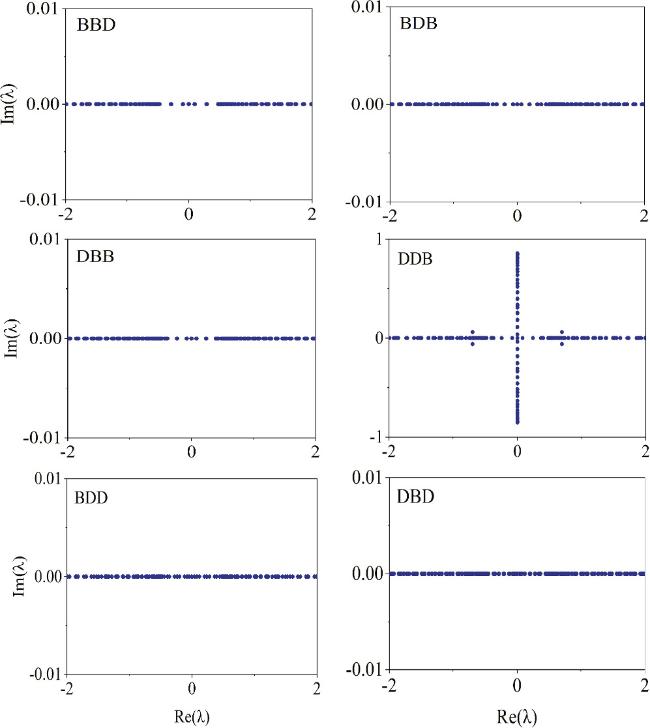
Figure 3. Bogoliubov–de Gennes excitation spectra of six types of spin solitons. BBD, BDB, and DBB exhibit a discrete spectrum without imaginary parts, while the DDB spectrum has non-zero imaginary parts and is unstable. When the G1 ≠ G2 spectra of BDD and DBD have non-zero imaginary parts, they are similar to that of DDB. When G1 = G2, BDD-2 and DBD-1 can admit continuous spectra without imaginary parts, which are shown in the lower panels. The parameters are the same as those in figure 2. |
The results of spectral stability analysis indicate that there are three types of spectra for the spin solitons, i.e. the discrete spectrum with a zero imaginary part, the discrete spectrum with a non-zero imaginary part and the continuous spectrum with a zero imaginary part. Next, we choose BBD, DDB and DBD as representatives to perform numerical simulations of equation (1 ) (with gs = 0.02) and observe the soliton dynamics. All the parameters are the same as we used in figures 2 and 3. The initial states are given by the exact solution we presented, and 1% random noise is added to each component. The results are shown in figure 4. It can be seen that BBD remains stable over a long evolutionary time (over 600 dimensionless units). However, not all spin solitons are stable during evolution. The Bogoliubov–de Gennes excitation spectrum indicates that DDB is dynamically unstable, since it admits non-zero imaginary parts. These soliton structures will be destroyed rapidly, even in the absence of random noise. If G1 ≠ G2, the spectra for DBD (or BDD) also exhibit non-zero imaginary parts and they are dynamically unstable. Besides, when G1 = G2, we notice that they have a continuous excitation spectrum without an imaginary part but sudden unstable behavior occurs. As shown in figure 4(c), the soliton is stable for about 100 dimensionless units and then the system abruptly becomes unstable. This sudden unstable behavior is quite different from that with imaginary parts on the excitation spectrum. Because DBD can remain stable for a long time but finally becomes unstable, we refer to these special dynamics of the spin soliton as metastable. This result may indicate that spectral stability is not a sufficient condition for soliton stability during time evolution.

Figure 4. The evolutions of (a) BBD, (b) DDB and (c) DBD according to the original equation ( |
4. Collisions between spin solitons
In this section, we investigate the collision between two spin solitons. Due to the non-integrability of the model, exact two-spin soliton solutions cannot be obtained using the analytical methods [37–40]. Therefore, we study the collision process using numerical simulations. As an example, we demonstrate the collision between two BBDs. The initial state can be given by a linear superposition of two spin soliton solutions when they are placed far from each other,
$\begin{eqnarray}\begin{array}{rcl}{\psi }_{1} & = & {c}_{1}\sqrt{\displaystyle \frac{{F}_{2}-{F}_{4}}{{F}_{4}^{2}-{F}_{1}{F}_{2}}}{\kappa }_{1}{\rm{sech}} [{\kappa }_{1}(x-{x}_{10})]{{\rm{e}}}^{{\rm{i}}[{v}_{1}(x-{x}_{10})+{\rm{\Delta }}\phi ]}\\ & & +{c}_{2}\sqrt{\displaystyle \frac{{F}_{2}-{F}_{4}}{{F}_{4}^{2}-{F}_{1}{F}_{2}}}{\kappa }_{2}{\rm{sech}} [{\kappa }_{2}(x-{x}_{20})]{{\rm{e}}}^{{\rm{i}}[{v}_{2}(x-{x}_{20})},\end{array}\end{eqnarray}$
$\begin{eqnarray}\begin{array}{rcl}{\psi }_{2} & = & {c}_{2}\sqrt{\displaystyle \frac{{F}_{1}-{F}_{4}}{{F}_{4}^{2}-{F}_{1}{F}_{2}}}{\kappa }_{1}{\rm{sech}} [{\kappa }_{1}(x-{x}_{10})]{{\rm{e}}}^{{\rm{i}}[{v}_{1}(x-{x}_{10})+{\rm{\Delta }}\phi ]}\\ & & +{c}_{1}\sqrt{\displaystyle \frac{{F}_{1}-{F}_{4}}{{F}_{4}^{2}-{F}_{1}{F}_{2}}}{\kappa }_{2}{\rm{sech}} [{\kappa }_{2}(x-{x}_{20})]{{\rm{e}}}^{{\rm{i}}[{v}_{2}(x-{x}_{20})]},\end{array}\end{eqnarray}$
$\begin{eqnarray}\begin{array}{l}{\psi }_{3}=\left(\displaystyle \frac{1}{\sqrt{{F}_{3}}}\left\{{v}_{1}-{\rm{i}}{\kappa }_{1}\tanh [{\kappa }_{1}(x-{x}_{10})]\right\}\right)\\ \,\times \,\left(\displaystyle \frac{1}{\sqrt{{F}_{3}}}\left\{{v}_{2}-{\rm{i}}{\kappa }_{2}\tanh [{\kappa }_{2}(x-{x}_{20})]\right\}\right).\end{array}\end{eqnarray}$
The parameters ${\kappa }_{l}=\sqrt{{F}_{3}-{v}_{l}^{2}}$ (l = 1,2) represent the inverse widths of two spin solitons, and xl0 determine the initial positions of two solitons. The Δφ denotes the relative phase between bright solitons. By adjusting vl, one can investigate collisions between spin solitons with different velocities.
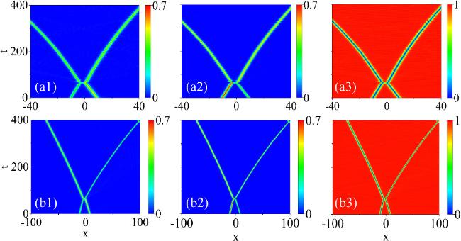
In figures 5(a1)–(a3), we illustrate one case with v1 = − v2 = 0.1 and Δφ = 0. When the soliton velocity is much lower than the maximum speed, mass transport between bright solitons leads to changes in soliton profiles after the collision. In figures 5(b1)–(b3), we present the case where Δφ = π/2, while the velocities are retained. The relative phase between two bright solitons significantly changes the density redistribution during the collision. This phenomenon is similar to that reported in [34]. Interestingly, spin solitons exhibit weak amplitude and positional oscillations and accelerating behavior after collisions in both cases. The shape oscillation arises due to the presence of pairs of internal modes in the spectrum of spin solitons in the non-integrable model, and it causes resonant energy radiation [52, 53]. As a consequence, the soliton energy decreases, leading to the acceleration of spin solitons. Since the oscillation frequency and energy radiation are much lower, this phenomenon was not observed in [34].
Figure 5. The density redistribution and weak oscillations after the collision between two BBDs. The soliton speeds are much lower than the maximum speed. (a1)–(a3) depict the case with velocities v1 = −v2 = 0.1 and a relative phase Δφ = 0; (b1)–(b3) v1 = −v2 = 0.1 but Δφ = π/2. It can be observed that the density redistribution occurs in both cases and it can be changed by the relative phase of bright solitons. After the collisions, spin solitons experience weak shape oscillations, which are induced by the non-integrability of the system. The nonlinear coefficients are the same as those in figure 2, and the other parameters are: ${c}_{1}=\sqrt{2/3}$, ${c}_{2}=\sqrt{1/3}$, x10 = −10 and x20 = 10. |
When the speeds of two spin solitons approach the maximum speed, the collisions between them are almost elastic and the relative phase only changes the interference patterns in the collision process, which is similar to that reported in [34]. Numerical simulations show that the collisions for the other two types of spin solitons (BDB and DBB) are similar to those of BBD. During the collisions, the spin density undergoes redistribution and the non-integrability of the system induces weak oscillations and an acceleration phenomenon after collisions.
5. Conclusions
We obtain six types of exact analytical spin soliton solutions that exist in the extended region of nonlinearity coefficient space. These results further enrich the soliton solutions for the spin-1 BEC systems. By analysing the Bogoliubov–de Gennes excitation spectra and performing numerical simulations of these spin solitons, three types of spin solitons are confirmed to be stable against small deviations caused by spin-dependent terms and weak noise. In particular, two types of spin solitons are shown to be spectrally stable but become unstable over a rather long time period. We therefore refer to this novel case as metastable. The collisions between spin solitons directly exhibit the non-integrability of the model. Spin solitons start oscillation after the collision, and the energy radiation caused by the oscillation results in the acceleration of solitons. These results further enrich the soliton family for non-integrable models and can provide theoretical references for the experimental observation of spin solitons.
Appendix. Decoupling method
The coupled Gross–Pitaevskii equations (equation (1 )) can be reduced to the following equations when the external potentials are Vi(x) = 0 and the weak spin-dependent effects are ignored,
$\begin{eqnarray}{\rm{i}}\displaystyle \frac{\partial {\psi }_{1}}{\partial t}=-\displaystyle \frac{1}{2}\displaystyle \frac{{\partial }^{2}{\psi }_{1}}{\partial {x}^{2}}-({g}_{11}| {\psi }_{1}{| }^{2}+{g}_{12}| {\psi }_{2}{| }^{2}+{g}_{13}| {\psi }_{3}{| }^{2}){\psi }_{1},\end{eqnarray}$
$\begin{eqnarray}{\rm{i}}\displaystyle \frac{\partial {\psi }_{2}}{\partial t}=-\displaystyle \frac{1}{2}\displaystyle \frac{{\partial }^{2}{\psi }_{2}}{\partial {x}^{2}}-({g}_{21}| {\psi }_{1}{| }^{2}+{g}_{22}| {\psi }_{2}{| }^{2}+{g}_{23}| {\psi }_{3}{| }^{2}){\psi }_{2},\end{eqnarray}$
$\begin{eqnarray}{\rm{i}}\displaystyle \frac{{\rm{\partial }}{\psi }_{3}}{{\rm{\partial }}t}=-\displaystyle \frac{1}{2}\displaystyle \frac{{{\rm{\partial }}}^{2}{\psi }_{3}}{{\rm{\partial }}{x}^{2}}-({g}_{31}|{\psi }_{1}{|}^{2}+{g}_{32}|{\psi }_{2}{|}^{2}+{g}_{33}|{\psi }_{3}{|}^{2}){\psi }_{3}.\end{eqnarray}$
By introducing the constraints on total density for spin solitons (∑∣ψi∣2 = 1) and the nonlinearity coefficients (g13 = g23), equation (A1 ) can be written as follows:A2 ) can be further simplified to:
$\begin{eqnarray}\begin{array}{l}{\rm{i}}\displaystyle \frac{\partial {\psi }_{1}}{\partial t}=-\displaystyle \frac{1}{2}\displaystyle \frac{{\partial }^{2}{\psi }_{1}}{\partial {x}^{2}}-[({g}_{11}-{G}_{2})| {\psi }_{1}{| }^{2}\\ \quad +({G}_{1}-{G}_{2})| {\psi }_{2}{| }^{2}]{\psi }_{1}-{G}_{2}{\psi }_{1},\end{array}\end{eqnarray}$
$\begin{eqnarray}\begin{array}{l}{\rm{i}}\displaystyle \frac{\partial {\psi }_{2}}{\partial t}=-\displaystyle \frac{1}{2}\displaystyle \frac{{\partial }^{2}{\psi }_{2}}{\partial {x}^{2}}-[({G}_{1}-{G}_{2})| {\psi }_{1}{| }^{2}\\ \quad +({g}_{22}-{G}_{2})| {\psi }_{2}{| }^{2}]{\psi }_{2}-{G}_{2}{\psi }_{2},\end{array}\end{eqnarray}$
$\begin{eqnarray}{\rm{i}}\displaystyle \frac{\partial {\psi }_{3}}{\partial t}=-\displaystyle \frac{1}{2}\displaystyle \frac{{\partial }^{2}{\psi }_{3}}{\partial {x}^{2}}-({g}_{33}-{G}_{2})| {\psi }_{3}{| }^{2}{\psi }_{3}-{G}_{2}{\psi }_{3},\end{eqnarray}$
where G1 = g12 = g21 and G2 = g13 = g31 = g23 = g32. By taking ${\psi }_{i}={q}_{i}{{\rm{e}}}^{{\rm{i}}{G}_{2}t}$, equation ( $\begin{eqnarray}{\rm{i}}\displaystyle \frac{\partial {q}_{1}}{\partial t}+\displaystyle \frac{1}{2}\displaystyle \frac{{\partial }^{2}{q}_{1}}{\partial {x}^{2}}-({F}_{1}| {q}_{1}{| }^{2}+{F}_{4}| {q}_{2}{| }^{2}){q}_{1}=0,\end{eqnarray}$
$\begin{eqnarray}{\rm{i}}\displaystyle \frac{\partial {q}_{2}}{\partial t}+\displaystyle \frac{1}{2}\displaystyle \frac{{\partial }^{2}{q}_{2}}{\partial {x}^{2}}-({F}_{4}| {q}_{1}{| }^{2}+{F}_{2}| {q}_{2}{| }^{2}){q}_{2}=0,\end{eqnarray}$
$\begin{eqnarray}{\rm{i}}\displaystyle \frac{\partial {q}_{3}}{\partial t}+\displaystyle \frac{1}{2}\displaystyle \frac{{\partial }^{2}{q}_{3}}{\partial {x}^{2}}-{F}_{3}| {q}_{3}{| }^{2}{q}_{3}=0,\end{eqnarray}$
where F1 = G2 − g11, F2 = G2 − g22, F3 = G2 − g33 and F4 = G2 − G1. By employing this approach, the original model is simplified into the form that consists of two-component coupled nonlinear Schrödinger equations (NLSEs) and a scalar NLSE. Since the exact soliton solutions for the non-integrable two-component NLSE (depart from the integrable limit F1 = F2 = F4) were obtained recently [26], we can greatly extend the existence region for the spin solitons [34]. When F3 takes a positive(negative) value, the third component admits a dark(bright) soliton solution. Considering the constraint on the total mass density ∑∣qi∣2 = 1, the mass density of the two-component coupled NLSE should admit a density hump (dip). Based on the soliton solutions in [26], the spin soliton solutions can be constructed.For example, we present how to obtain BBD. If F3 > 0, ∣q3∣2 is a dark soliton:A3 ):3 )–(5 )) of equation (A1 ) is obtained. Other types of spin solitons can also be derived by this method.
$\begin{eqnarray}{q}_{3D}=\displaystyle \frac{1}{\sqrt{{F}_{3}}}\left\{v-{\rm{i}}\sqrt{{F}_{3}-{v}^{2}}\tanh [\sqrt{{F}_{3}-{v}^{2}}(x-{vt})]\right\}{{\rm{e}}}^{-{\rm{i}}{F}_{3}t}.\end{eqnarray}$
To keep the total mass density uniform (∑∣qi∣2=1), the two coupled components (∣q1∣2 + ∣q2∣2) should be a ‘bright soliton'. Therefore, we set F1 > F4, F2 > F4, and the coupled q1 and q2 admit a bright-bright soliton [26]: $\begin{eqnarray}{q}_{1B}={f}_{1}{\rm{sech}} [w(x-{vt})]{{\rm{e}}}^{{\rm{i}}[\tfrac{1}{2}({w}^{2}+{v}^{2})t+(x-{vt})v]},\end{eqnarray}$
$\begin{eqnarray}{q}_{2B}={f}_{2}{\rm{sech}} [w(x-{vt})]{{\rm{e}}}^{{\rm{i}}[\tfrac{1}{2}({w}^{2}+{v}^{2})t+(x-{vt})v]},\end{eqnarray}$
where $w=\sqrt{({F}_{2}-{F}_{4})/({F}_{4}^{2}-{F}_{1}{F}_{2})}{f}_{1}$, and ${f}_{2}=\sqrt{({F}_{4}-{F}_{1})/({F}_{4}-{F}_{2})}{f}_{1}$. According to the restriction on the total mass density, one can obtain the conditions of $\sqrt{{F}_{3}-{v}^{2}}=\sqrt{({F}_{2}-{F}_{4})/({F}_{4}^{2}-{F}_{1}{F}_{2})}{f}_{1}$ and ${f}_{1}^{2}+{f}_{2}^{2}=({F}_{3}-{v}^{2})/{F}_{3}$ and then get the expression of f1 and f2. Therefore, we can obtain the solution for equation ( $\begin{eqnarray}{q}_{1B}=\sqrt{\displaystyle \frac{{F}_{2}-{F}_{4}}{{F}_{4}^{2}-{F}_{1}{F}_{2}}}w{\rm{sech}} [w(x-{vt})]{{\rm{e}}}^{{\rm{i}}[\tfrac{1}{2}({w}^{2}+{v}^{2})t+(x-{vt})v]},\end{eqnarray}$
$\begin{eqnarray}{q}_{2B}=\sqrt{\displaystyle \frac{{F}_{1}-{F}_{4}}{{F}_{4}^{2}-{F}_{1}{F}_{2}}}w{\rm{sech}} [w(x-{vt})]{{\rm{e}}}^{{\rm{i}}[\tfrac{1}{2}({w}^{2}+{v}^{2})t+(x-{vt})v]},\end{eqnarray}$
$\begin{eqnarray}{q}_{3D}=\displaystyle \frac{1}{\sqrt{{F}_{3}}}\left\{v-{\rm{i}}w\tanh [w(x-{vt})]\right\}{{\rm{e}}}^{-{\rm{i}}{F}_{3}t},\end{eqnarray}$
where $w=\sqrt{{F}_{3}-{v}^{2}}$. Finally, by taking ${\psi }_{i}={q}_{i}{{\rm{e}}}^{{\rm{i}}{G}_{2}t}$, the BBD solution (equations (