


1. Introduction
Over the past few decades, various kinds of techniques have been successively proposed for investigating the solutions and properties of the NLEEs, including the bilinear method [8], Darboux transformation method [9–11], Bäcklund transformation method (BT) [12], Painlevé analysis method [13], inverse scattering transformation method (IST) [14, 15], the Exp-function method [16], the homogeneous balance method [17], the tanh and extended tanh methods [18–20], Lax pair method [21] and Lie symmetry method [22, 23], etc.
As an important prototypical NLEE, the modified Korteweg–de Vries (mKdV) equation [24, 25]
$\begin{eqnarray}{u}_{t}-6{u}^{2}\,{u}_{x}+{u}_{{xxx}}=0\end{eqnarray}$
is one of the most fundamental modified versions of KdV equation, with the sign of the cubic nonlinearity negative, and in such condition there exists the Miura transformation connecting the mKdV equation with the KdV one [5].The modified Kadomtsev–Petviashvili (mKP) equation [26] is a two-spatial dimensional analog of mKdV equation (1 ),2 ) can describe the propagation of electromagnetic waves in an isotropic charge-free infinite ferromagnetic thin film [3, 26–28] and water wave in the x − y plane when the nonlinearity is higher than the KP equation [29], general nonlinear wave phenomena exhibiting cubic nonlinearity, dispersion and small transversality in (2+1) dimensions [30], nonlinear wave in the plasma physics and electrodynamics [4, 31].
$\begin{eqnarray}\left\{\begin{array}{l}{u}_{t}-6{u}^{2}\,{u}_{x}+{u}_{{xxx}}-3\alpha (2v\,{u}_{x}-\alpha \,{v}_{y})=0,\\ {u}_{y}={v}_{x},\end{array}\right.\end{eqnarray}$
where x, y are space coordinates, t is a temporal coordinate and α is an arbitrary constant. Equation (Many novel results in solutions of the mKP equation (2 ) have been constructed in recent years. The N-front wave solutions have been obtained by the perturbation expansion method [4]. Two graded symmetry Lie algebras for modified KP equations have been obtained [32]. Lie algebraic structures of the scalar mKP flows have been investigated [33]. Some special types of the multi-soliton solutions of equation (2 ) have been provided by using the standard truncated Painlevé analysis approach [34], and the interaction between kink solitons and line solitons have been investigated via the τ-function and the Binet–Cauchy formula [35]. For the variable-coefficient mKP equation, the Painlevé test has been used to find the necessary integrability conditions, Bäcklund transformation has been given to find kink solitary wave solution, and N-soliton solutions have been obtained for the vcmKP system [36]. The obtained integrability conditions from Compatible Riccati Expansion (CRE) solvability have shown a (3+1)-dimensional variable-coefficient mKP system and novel shock, solitary and periodic wave solutions have been obtained from both CRE and the direct reduction method [37].
When the media are inhomogeneous or the boundaries are nonuniform, the variable-coefficient models are able to describe various situations more realistically than their constant-coefficient counterparts [38]. In this paper, we will focus our attention on a variable-coefficient modified Kadomtsev–Petviashvili (vcmKP) equation [39], a generalized case of equation (2 ) from fluids and plasma [40],
$\begin{eqnarray}\left\{\begin{array}{l}{u}_{t}-6{u}^{2}\,{u}_{x}+{u}_{{xxx}}+{a}_{1}v\,{u}_{x}+{a}_{2}\,{v}_{y}+{b}_{1}(t){u}_{x}+{b}_{2}(t){u}_{y}=0,\\ {u}_{y}={v}_{x},\end{array}\right.\end{eqnarray}$
where a1, a2 are two arbitrary constants, b1(t) and b2(t) are two arbitrary functions of t, the real differentiable function u(x, y, t) standing for the first derivative of the angle made between the propagation direction for the electromagnetic wave and direction for the uniform magnetization of the medium with respect to x, v(x, y, t) meaning a real differentiable function, x representing the stretched wave variable with the assumption that the electromagnetic wave propagates along the x direction on the x − y plane, y denoting the scaled stretched variable along the normal y direction, t indicating the scaled stretched time [36].The structure of this paper is listed as follows. In section 2 , the Painlevé test will be applied to equation (3 ) in order to obtain Painlevé integrable conditions, auto-Bäcklund transformation will be presented via the truncated Painlevé expansion, and analytic solutions will be provided, including the solitonic, periodic and rational solutions. In section 3 , the infinitesimal generators and symmetry groups of equation (3 ) will be presented by the Lie group method. In section 4 , the optimal system and similarity reductions to partial differential equations (PDEs) will be obtained, with some similarity solutions provided. In section 4 , by virtue of symbolic computation, nonlinear self-adjointness for equation (3 ) will be presented. Based on the nonlinear self-adjointness, an infinite number of conservation laws will be derived with a general conservation. Conclusions and discussions are given in the last section.
2. Painlevé property, auto-Bäcklund transformation and analytic solutions
2.1. Painlevé property
We assume solutions of equation (3 ) have the form of the following generalized Laurent expansion [41, 42],
$\begin{eqnarray}\begin{array}{rcl}u(x,y,t) & = & {\phi }^{\,p}(x,y,t)\displaystyle \sum _{j=0}^{\infty }{u}_{j}(y,t){\phi }^{\,j}(x,y,t),\\ v(x,y,t) & = & {\phi }^{\,q}(x,y,t)\displaystyle \sum _{j=0}^{\infty }{v}_{j}(y,t){\phi }^{\,j}(x,y,t),\end{array}\end{eqnarray}$
with φ(x, y, t) = x + ψ(y, t),where ψ(y, t) is an arbitrary function of y and t, and uj(y, t), vj(y, t)(j = 0, 1, 2, ⋯ ) are all analytic functions of y and t, in the neighborhood of a noncharacteristic movable singularity manifold defined by φ(x, y, t) = 0.By the leading-order analysis, one can get3 ) possesses the Painlevé property if and only if
$\begin{eqnarray}p=1,q=1,{u}_{0}=\pm 1,{v}_{0}=\mp {\psi }_{y}.\end{eqnarray}$
It is found that the resonances occur at j = − 1, 1, 3, 4, and equation ( $\begin{eqnarray}{a}_{2}=\displaystyle \frac{1}{12}{a}_{1}^{2},\end{eqnarray}$
while coefficient functions b1(t) and b2(t) are free.Without losing generality, we set a1 = − 6α, a2 = 3α2 in equation (3 ) in the next investigation.
2.2. Auto-Bäcklund transformation and analytic solutions
Bäcklund transformation connects the solutions of two differential equations, i.e. if the solution of one equation is known, the solution of the other equation can be obtained by this transformation. In particular, if both solutions of the transformation are of the same equation, it is called the auto-Bäcklund transformation of equation [45].
Taking the general form φ = φ(x, y, t) in equation (4 ) and u1 = 0, v1 = 0 as the seed solutions and truncating the Painlevé expansion at the constant-level term, one can get the following auto-Bäcklund transformation for the vcmKP equation (3 ):
$\begin{eqnarray}u={\left(\mathrm{ln}\,\phi \right)}_{x},v={\left(\mathrm{ln}\,\phi \right)}_{y},\end{eqnarray}$
where φ(x, y, t) satisfies the following equations, $\begin{eqnarray}{\phi }_{{xx}}+\alpha {\phi }_{y}=0,\end{eqnarray}$
$\begin{eqnarray}{\phi }_{t}+4{\phi }_{{xxx}}+{b}_{1}(t){\phi }_{x}+{b}_{2}(t){\phi }_{y}=0.\end{eqnarray}$
We are going to find the solutions in the form
$\begin{eqnarray}\phi =1+H(\rho )\,{{\rm{e}}}^{\theta }=1+H\,[k\,x+m\,y+l(t)]\,\,{{\rm{e}}}^{p\,x+r\,y+s(t)},\end{eqnarray}$
where k, m, p and r are all constants, l(t) and s(t) are functions of t, whereas function H(ρ) may be sine, cosine, hyperbolic cosine, hyperbolic sine and so on. Now, we consider some special situations.Case 1 H(ρ) = 1
In this case, the general solution reads
$\begin{eqnarray}\begin{array}{rcl}{\phi }_{1} & = & 1+\,{{\rm{e}}}^{\theta },\ \ \ \theta =p\,x+r\,y+s(t)=p\,x-\displaystyle \frac{{p}^{2}}{\alpha }y\\ & & +\displaystyle \int \left[\displaystyle \frac{{p}^{2}{b}_{2}(t)}{\alpha }-4{p}^{3}-{{pb}}_{1}(t)\right]{\rm{d}}t.\end{array}\end{eqnarray}$
Case 2 $H(\rho )=\cosh (\rho )$ or $H(\rho )=\sinh (\rho )$After some calculation with symbolic computation, we obtain the solutions
$\begin{eqnarray}{\phi }_{2}=1+\cosh (\rho )\,{{\rm{e}}}^{\theta },\end{eqnarray}$
$\begin{eqnarray}{\phi }_{3}=1+\sinh (\rho )\,{{\rm{e}}}^{\theta },\end{eqnarray}$
where $\begin{eqnarray*}\begin{array}{rcl}\rho & = & {kx}-\displaystyle \frac{2{kp}}{\alpha }y+\displaystyle \int \left[\displaystyle \frac{2{kp}}{\alpha }{b}_{2}(t)-{{kb}}_{1}(t)\right.\\ & & \left.-4{k}^{3}-12{{kp}}^{2}\Space{0ex}{2.85ex}{0ex}\right]{\rm{d}}t,\\ \theta & = & {px}-\displaystyle \frac{{k}^{2}\,+\,{p}^{2}}{\alpha }y+\displaystyle \int \left[\displaystyle \frac{{k}^{2}+{p}^{2}}{\alpha }{b}_{2}(t)\right.\\ & & \left.-{{pb}}_{1}(t)-4{p}^{3}-12{{pk}}^{2}\Space{0ex}{2.85ex}{0ex}\right]{\rm{d}}t.\end{array}\end{eqnarray*}$
Case 3 $H(\rho )=\cos (\rho )$ or $H(\rho )=\sin (\rho )$Similarly, we get the solutions
$\begin{eqnarray}{\phi }_{4}=1+\cos (\rho )\,{{\rm{e}}}^{\theta },\end{eqnarray}$
$\begin{eqnarray}{\phi }_{5}=1+\sin (\rho )\,{{\rm{e}}}^{\theta },\end{eqnarray}$
where $\begin{eqnarray*}\begin{array}{rcl}\rho & = & {kx}-\displaystyle \frac{2{kp}}{\alpha }y\\ & & +\ \displaystyle \int \left[\displaystyle \frac{2{kp}}{\alpha }{b}_{2}(t)-{{kb}}_{1}(t)+4{k}^{3}-12{{kp}}^{2}\right]{\rm{d}}t,\\ \theta & = & {px}+\displaystyle \frac{{k}^{2}-{p}^{2}}{\alpha }y\\ & & +\ \displaystyle \int \left[\displaystyle \frac{{p}^{2}-{k}^{2}}{\alpha }{b}_{2}(t)-{{pb}}_{1}(t)-4{p}^{3}+12{{pk}}^{2}\right]{\rm{d}}t.\end{array}\end{eqnarray*}$
Because equations (8 ) and (9 ) are linear, some kinds of solutions φ listed above may be combined appropriately, and different kinds of solutions φ can be combined to form some new kinds of analytic solutions,
$\begin{eqnarray}\begin{array}{rcl}{\phi }_{6} & = & 1+\displaystyle \sum _{i=0}^{{N}_{1}}{d}_{i}^{(1)}\,{{\rm{e}}}^{{\theta }_{i}^{{\prime} }}+\displaystyle \sum _{i=0}^{{N}_{2}}{d}_{i}^{(2)}\cosh ({\rho }_{i}^{{\prime\prime} })\,{{\rm{e}}}^{{\theta }_{i}^{{\prime\prime} }}\\ & & +\ \displaystyle \sum _{i=0}^{{N}_{3}}{d}_{i}^{(3)}\sinh ({\rho }_{i}^{{\prime\prime} })\,{{\rm{e}}}^{{\theta }_{i}^{{\prime\prime} }}\\ & & +\ \displaystyle \sum _{i=0}^{{N}_{4}}{d}_{i}^{(4)}\cos ({\rho }_{i}^{\prime\prime\prime })\,{{\rm{e}}}^{{\theta }_{i}^{\prime\prime\prime }}+\displaystyle \sum _{i=0}^{{N}_{5}}{d}_{i}^{(5)}\sin ({\rho }_{i}^{\prime\prime\prime })\,{{\rm{e}}}^{{\theta }_{i}^{\prime\prime\prime }},\end{array}\end{eqnarray}$
where $\begin{eqnarray*}\begin{array}{rcl}{\theta }_{i}^{{\prime} } & = & {p}_{i}\,x-\displaystyle \frac{{p}_{i}^{2}}{\alpha }y+\displaystyle \int \left[\displaystyle \frac{{p}_{i}^{2}{b}_{2}(t)}{\alpha }-4{p}_{i}^{3}-{p}_{i}{b}_{1}(t)\right]{\rm{d}}t,\\ {\rho }_{i}^{{\prime\prime} } & = & {k}_{i}x-\displaystyle \frac{2{k}_{i}{p}_{i}}{\alpha }y\\ & & +\ \displaystyle \int \left[\displaystyle \frac{2{k}_{i}{p}_{i}}{\alpha }{b}_{2}(t)-{k}_{i}{b}_{1}(t)-4{k}_{i}^{3}-12{k}_{i}{p}_{i}^{2}\right]{\rm{d}}t,\\ {\theta }_{i}^{{\prime\prime} } & = & {p}_{i}x-\displaystyle \frac{{k}_{i}^{2}+{p}_{i}^{2}}{\alpha }y\\ & & +\ \displaystyle \int \left[\displaystyle \frac{{k}_{i}^{2}+{p}_{i}^{2}}{\alpha }{b}_{2}(t)-{p}_{i}{b}_{1}(t)-4{p}_{i}^{3}-12{p}_{i}{k}_{i}^{2}\right]{\rm{d}}t,\\ {\rho }_{i}^{\prime\prime\prime } & = & {k}_{i}x-\displaystyle \frac{2{k}_{i}{p}_{i}}{\alpha }y\\ & & +\ \displaystyle \int \left[\displaystyle \frac{2{k}_{i}{p}_{i}}{\alpha }{b}_{2}(t)-{k}_{i}{b}_{1}(t)+4{k}_{i}^{3}-12{k}_{i}{p}_{i}^{2}\right]{\rm{d}}t,\\ {\theta }_{i}^{\prime\prime\prime } & = & {p}_{i}x+\displaystyle \frac{{k}_{i}^{2}-{p}_{i}^{2}}{\alpha }y\\ & & +\ \displaystyle \int \left[\displaystyle \frac{{p}_{i}^{2}-{k}_{i}^{2}}{\alpha }{b}_{2}(t)-{p}_{i}{b}_{1}(t)-4{p}_{i}^{3}+12{p}_{i}{k}_{i}^{2}\right]{\rm{d}}t,\end{array}\end{eqnarray*}$
where the parameters ${d}_{i}^{(j)},{k}_{i},{p}_{i}\,(i=0,1,\ldots ,{N}_{j};\,{N}_{j}\geqslant 0,j=1,\cdots ,5)$ are all arbitrary constants.Thus the corresponding analytic solutions of equation (3 ) read as
$\begin{eqnarray}{u}_{i}={\left(\mathrm{ln}\,{\phi }_{i}\right)}_{x},{v}_{i}={\left(\mathrm{ln}\,{\phi }_{i}\right)}_{y},\qquad i=1,2,\cdots ,6.\end{eqnarray}$
In addition, we here provide one family rational solution as bellow,
$\begin{eqnarray*}\begin{array}{rcl}u & = & {\left(\mathrm{ln}\,\phi \right)}_{x},v={\left(\mathrm{ln}\,\phi \right)}_{y},\\ {\phi }_{7} & = & {c}_{4}{x}^{3}+{f}_{2}(t){x}^{2}+{f}_{1}(t)x+{f}_{0}(t)+\left[-\displaystyle \frac{6{c}_{4}}{\alpha }x+{g}_{0}(t)\right]y,\end{array}\end{eqnarray*}$
where $\begin{eqnarray*}\begin{array}{rcl}{f}_{2}(t) & = & {c}_{3}-3{c}_{4}\displaystyle \int {b}_{1}(t)\,{\rm{d}}t,\\ {f}_{1}(t) & = & {c}_{2}+\displaystyle \int \left[\displaystyle \frac{6{c}_{4}{b}_{2}(t)}{\alpha }-2{b}_{1}(t){f}_{2}(t)\right]\,{\rm{d}}t,\\ {f}_{0}(t) & = & {c}_{1}-24{c}_{4}t+\displaystyle \int \left[\displaystyle \frac{2{b}_{2}(t){f}_{2}(t)}{\alpha }-{b}_{1}(t){f}_{1}(t)\right]\,{\rm{d}}t,\\ {g}_{0}(t) & = & -\displaystyle \frac{2{f}_{2}(t)}{\alpha }.\end{array}\end{eqnarray*}$
3. Lie symmetry analysis
The Lie symmetry method is a fundamental and powerful approach for finding closed-form solutions of all types of differential equations via the Lie transformations, which can help to reduce one PDF into a new one with less number of independent variables [22, 23, 46–50]. Based on infinitesimal generators from Lie transformations the conservation laws can be derived by employing the multiplier method [46]. The goal of this study is to provide the symmetry property, similarity reduction and conservation laws of equation (3 ). In this section, we will perform Lie symmetry analysis for equation (3 ).
If equation (3 ) is invariant under a one-parameter Lie group of point transformations [46]19 ) generates a symmetry of equation (3 ), and V must satisfy Lie symmetry condition
$\begin{eqnarray}\left\{\begin{array}{l}{x}^{* }=x+\varepsilon {\xi }^{x}(x,y,t,u,v)+O({\varepsilon }^{2}),\\ {y}^{* }=y+\varepsilon {\xi }^{y}(x,y,t,u,v)+O({\varepsilon }^{2}),\\ {t}^{* }=t+\varepsilon \tau (x,y,t,u,v)+O({\varepsilon }^{2}),\\ {u}^{* }=u+\varepsilon \eta (x,y,t,u,v)+O({\varepsilon }^{2}),\\ {v}^{* }=v+\varepsilon \,\omega (x,y,t,u,v)+O({\varepsilon }^{2}),\end{array}\right.\end{eqnarray}$
where ϵ is a small parameter and functions τ, ξx, ξy and η, ω are the infinitesimals depending on x, y, t and u, v. The corresponding infinitesimal generator is expressed as $\begin{eqnarray}\begin{array}{rcl}V & = & {\xi }^{x}(x,y,t,u,v)\displaystyle \frac{\partial }{\partial x}+{\xi }^{y}(x,y,t,u,v)\displaystyle \frac{\partial }{\partial y}\\ & & +\tau (x,y,t,u,v)\displaystyle \frac{\partial }{\partial t}+\eta (x,y,t,u,v)\displaystyle \frac{\partial }{\partial u}\\ & & +\omega (x,y,t,u,v)\displaystyle \frac{\partial }{\partial v},\end{array}\end{eqnarray}$
then the vector field ( $\begin{eqnarray}{\mathrm{pr}}^{(3)}V({E}_{1}){| }_{{E}_{1}=0}=0,\ {\mathrm{pr}}^{(1)}V({E}_{2}){| }_{{E}_{2}=0}=0,\end{eqnarray}$
where $\begin{eqnarray}\left\{\begin{array}{l}{E}_{1}={u}_{t}-6{u}^{2}\,{u}_{x}+{u}_{{xxx}}-3\alpha (2v\,{u}_{x}-\alpha \,{v}_{y})+{b}_{1}(t){u}_{x}+{b}_{2}(t){u}_{y},\\ {E}_{2}={u}_{y}-{v}_{x},\end{array}\right.\end{eqnarray}$
and pr(3)V, pr(1)V are the third and first prolongations of the infinitesimal generator V, respectively [46].Without loss of generality, we assume that ηv = ωu = 0. Expanding equation (20 ) and splitting the derivatives of u, v lead us to the following system of determining equations via symbolic computation,
$\begin{eqnarray}\left\{\begin{array}{l}{\xi }_{x}^{y}={\xi }_{y}^{x}={\tau }_{x}={\tau }_{y}={\eta }_{{uu}}=0,\\ {\eta }_{{xu}}-{\xi }_{{xx}}^{x}=0,\\ -{\xi }_{t}^{y}+{b}_{2}(t)(3{\xi }_{x}^{x}-{\xi }_{y}^{y})+\tau \,{b}_{2}^{\prime} (t)=0,\\ 3{\xi }_{x}^{x}-{\tau }_{t}=0,\\ {\omega }_{v}-{\xi }_{y}^{y}={\eta }_{u}-3{\xi }_{x}^{x},\\ {\omega }_{v}-{\xi }_{x}^{x}={\eta }_{u}-{\xi }_{y}^{y},\\ -{\xi }_{t}^{x}-{\xi }_{{xxx}}^{x}+3{\eta }_{{xxu}}-12{\xi }_{x}^{x}\,\alpha \,v-12{\xi }_{x}^{x}\,{u}^{2}+2{b}_{1}(t){\xi }_{x}^{x}-12u\,\eta -6\alpha \,\omega +\tau \,{b}_{1}^{\prime} (t)=0,\\ {\eta }_{t}-6{u}^{2}{\eta }_{x}+{\eta }_{{xxx}}-6\alpha \,v\,{\eta }_{x}+3{\alpha }^{2}\,{\omega }_{y}+{b}_{2}(t){\eta }_{y}+{b}_{1}(t){\eta }_{x}=0,\\ {\eta }_{y}={\omega }_{x}.\end{array}\right.\end{eqnarray}$
Solving the above equations yields the following infinitesimals,
$\begin{eqnarray}\left\{\begin{array}{l}{\xi }^{x}={c}_{1}\,x-6\alpha \,f(t)+3{c}_{1}\,t\,{b}_{1}(t)-{c}_{1}\displaystyle \int {b}_{1}(t){\rm{d}}t+{c}_{2}\,{b}_{1}(t)+{c}_{3},\\ {\xi }^{y}=2{c}_{1}\,y+3{c}_{1}\,t\,{b}_{2}(t)-2{c}_{1}\displaystyle \int {b}_{2}(t){\rm{d}}t+{c}_{2}\,{b}_{2}(t)+{c}_{4},\\ \tau =3{c}_{1}\,t+{c}_{2},\\ \eta =-{c}_{1}\,u,\\ \omega =-2{c}_{1}\,v+f^{\prime} (t),\end{array}\right.\end{eqnarray}$
where c1, c2, c3 are all arbitrary constants and f(t) is an arbitrary differentiable function of t.Thus, the Lie algebra of equation (3 ) is spanned via the following Lie symmetry generators
$\begin{eqnarray}\left\{\begin{array}{l}{V}_{1}=\displaystyle \frac{\partial }{\partial \,x},\\ {V}_{2}=\displaystyle \frac{\partial }{\partial \,y},\\ {V}_{3}={b}_{1}(t)\displaystyle \frac{\partial }{\partial \,x}+{b}_{2}(t)\displaystyle \frac{\partial }{\partial \,y}+\displaystyle \frac{\partial }{\partial \,t},\\ {V}_{4}=-6\alpha \,f(t)\displaystyle \frac{\partial }{\partial \,x}+f^{\prime} (t)\displaystyle \frac{\partial }{\partial \,v},\\ {V}_{5}=(x+3t\,{b}_{1}(t)-\displaystyle \int {b}_{1}(t)\,{\rm{d}}t)\displaystyle \frac{\partial }{\partial \,x}+(2y+3t\,{b}_{2}(t)-2\displaystyle \int {b}_{2}(t)\,{\rm{d}}t)\displaystyle \frac{\partial }{\partial \,y}+3t\,\displaystyle \frac{\partial }{\partial \,t}-u\,\displaystyle \frac{\partial }{\partial \,u}-2v\,\displaystyle \frac{\partial }{\partial \,v},\end{array}\right.\end{eqnarray}$
with f(t) being an arbitrary differentiable function.Hence one-parameter Lie symmetry groups G(ϵ) generated by Vi(i = 1, 2, ⋯ ,5) are
$\begin{eqnarray}{G}_{1}:(x,y,t,u,v)\to (x+\varepsilon ,y,t,u,v),\end{eqnarray}$
$\begin{eqnarray}{G}_{2}:(x,y,t,u,v)\to (x,y+\varepsilon ,t,u,v),\end{eqnarray}$
$\begin{eqnarray}\begin{array}{l}{G}_{3}:(x,y,t,u,v)\to (x+\displaystyle \int {b}_{1}(t+\varepsilon )-{b}_{1}(t){\rm{d}}t,y\\ \quad +\displaystyle \int {b}_{2}(t+\varepsilon )-{b}_{2}(t){\rm{d}}t,t+\varepsilon ,u,v),\end{array}\end{eqnarray}$
$\begin{eqnarray}{G}_{4}:(x,y,t,u,v)\to (x-6\,\alpha \,f(t)\varepsilon ,y,t,u,v+f^{\prime} (t)\varepsilon )\end{eqnarray}$
$\begin{eqnarray}\begin{array}{l} {G}_{5}:(x,y,t,u,v)\to (\,{{\rm{e}}}^{\varepsilon }(x-\displaystyle \int {b}_{1}(t){\rm{d}}t)\\ \quad +\,{{\rm{e}}}^{3\varepsilon }\,\displaystyle \int {b}_{1}(\,{{\rm{e}}}^{3\varepsilon }t){\rm{d}}t,\\ \,{{\rm{e}}}^{2\varepsilon }(y-\displaystyle \int {b}_{2}(t){\rm{d}}t)+\,{{\rm{e}}}^{3\varepsilon }\,\displaystyle \int {b}_{2}(\,{{\rm{e}}}^{3\varepsilon }t){\rm{d}}t,\end{array}\end{eqnarray}$
$\begin{eqnarray}\,{{\rm{e}}}^{3\varepsilon }\,t,\,{{\rm{e}}}^{-\varepsilon }\,u,\,{{\rm{e}}}^{-2\varepsilon }\,v).\end{eqnarray}$
Since Gi(i = 1, 2, ⋯ ,5) are symmetry groups, we can get the following theorem.
If {$u={f}_{1}(x,y,t),v={f}_{2}(x,y,t)$} is a solution of equation (
$\begin{eqnarray}({u}^{(1)},{v}^{(1)})=\left({f}_{1}(x-\varepsilon ,y,t),{f}_{2}(x-\varepsilon ,y,t)\right),\end{eqnarray}$
$\begin{eqnarray}({u}^{(2)},{v}^{(2)})=\left({f}_{1}(x,y-\varepsilon ,t),{f}_{2}(x,y-\varepsilon ,t)\right),\end{eqnarray}$
$\begin{eqnarray}\begin{array}{rcl}({u}^{(3)},{v}^{(3)}) & = & \left({f}_{1}(x-\displaystyle \int {b}_{1}(t)-{b}_{1}(t-\varepsilon ){\rm{d}}t,y\right.\\ & & -\displaystyle \int {b}_{2}(t)-{b}_{2}(t-\varepsilon ){\rm{d}}t,t-\varepsilon ),\end{array}\end{eqnarray}$
$\begin{eqnarray}\begin{array}{l}{f}_{2}(x-\displaystyle \int {b}_{1}(t)-{b}_{1}(t-\varepsilon ){\rm{d}}t,y\\ \quad \left.-\displaystyle \int {b}_{2}(t)-{b}_{2}(t-\varepsilon ){\rm{d}}t,t-\varepsilon )\right),\end{array}\end{eqnarray}$
$\begin{eqnarray}\begin{array}{l}({u}^{(4)},{v}^{(4)})=\left({f}_{1}(x+6\,\alpha \,f(t)\varepsilon ,y,t),{f}_{2}(x\right.\\ \quad \left.+6\,\alpha \,f(t)\varepsilon ,y,t)+f^{\prime} (t)\varepsilon \right),\end{array}\end{eqnarray}$
$\begin{eqnarray}\begin{array}{rcl}({u}^{(5)},{v}^{(5)}) & = & \left(\,{{\rm{e}}}^{-\varepsilon }\,{f}_{1}\left[\,{{\rm{e}}}^{-\varepsilon }(x-\displaystyle \int {b}_{1}(\,{{\rm{e}}}^{3\varepsilon }t){\rm{d}}(\,{{\rm{e}}}^{3\varepsilon }t))\right.\right.\\ & & +\displaystyle \int {b}_{1}(t){\rm{d}}t,\,{{\rm{e}}}^{-2\varepsilon }(y-\displaystyle \int {b}_{2}(\,{{\rm{e}}}^{3\varepsilon }t){\rm{d}}(\,{{\rm{e}}}^{3\varepsilon }t))\\ & & \left.+\displaystyle \int {b}_{2}(t){\rm{d}}t,\,{{\rm{e}}}^{-3\varepsilon }\,t\right],\end{array}\end{eqnarray}$
$\begin{eqnarray}\begin{array}{l}\,{{\rm{e}}}^{-2\varepsilon }\,{f}_{2}\left[\,{{\rm{e}}}^{-\varepsilon }(x-\displaystyle \int {b}_{1}(\,{{\rm{e}}}^{3\varepsilon }t){\rm{d}}(\,{{\rm{e}}}^{3\varepsilon }t))\right.\\ \quad +\displaystyle \int {b}_{1}(t){\rm{d}}t,\,{{\rm{e}}}^{-2\varepsilon }(y-\displaystyle \int {b}_{2}(\,{{\rm{e}}}^{3\varepsilon }t){\rm{d}}(\,{{\rm{e}}}^{3\varepsilon }t))\\ \quad \left.\left.+\displaystyle \int {b}_{2}(t){\rm{d}}t,\,{{\rm{e}}}^{-3\varepsilon }\,t\right]\right).\end{array}\end{eqnarray}$
The Lie algebra commutator table is shown in table 1, where Lie bracket [Vi, Vj] = ViVj − VjVi.
Table 1. Commutator table of equation ( |
| [Vi, Vj] | V1 | V2 | V3 | V4 | V5 |
|---|---|---|---|---|---|
| V1 | 0 | 0 | 0 | 0 | V1 |
| V2 | 0 | 0 | 0 | 0 | 2V2 |
| V3 | 0 | 0 | 0 | V4 | 3V3 |
| V4 | 0 | 0 | −V4 | 0 | V4 |
| V5 | −V1 | −2V2 | −3V3 | −V4 | 0 |
4. Nonlinear self-adjointness and conservation laws
4.1. Nonlinear self-adjointness
To investigate its self-adjointness [51, 52], let the vcmKP equation (3 ) be noted as3 )40 )38 ) and (39 ). By comparing the coefficients of each term of (43-1 ) and (43-2 ) it is obtained that
$\begin{eqnarray}\begin{array}{rcl}{E}_{1} & = & {u}_{t}-6{u}^{2}\,{u}_{x}+{u}_{{xxx}}-3\alpha (2v\,{u}_{x}-\alpha \,{v}_{y})\\ & & +{b}_{1}(t){u}_{x}+{b}_{2}(t){u}_{y},\end{array}\end{eqnarray}$
$\begin{eqnarray}{E}_{2}={u}_{y}-{v}_{x}.\end{eqnarray}$
Then we have the following formal Lagrangian for equation ( $\begin{eqnarray}\begin{array}{rcl}{ \mathcal L } & = & \overline{u}\,{E}_{1}+\overline{v}\,{E}_{2}=\overline{u}\,[{u}_{t}-6{u}^{2}\,{u}_{x}+{u}_{{xxx}}\\ & & -3\alpha (2v\,{u}_{x}-\alpha \,{v}_{y})\\ & & +{b}_{1}(t){u}_{x}+{b}_{2}(t){u}_{y}]+\overline{v}({u}_{y}-{v}_{x}).\end{array}\end{eqnarray}$
To compute the variational derivative of the formal Lagrangian ( $\begin{eqnarray}\begin{array}{rcl}{E}_{1}^{* } & = & \displaystyle \frac{\delta ({ \mathcal L })}{\delta \,u}\\ & = & \left(\displaystyle \frac{\partial }{\partial u}-{D}_{t}\,\displaystyle \frac{\partial }{\partial {u}_{t}}\right.\\ & & \left.-{D}_{x}\,\displaystyle \frac{\partial }{\partial {u}_{x}}-{D}_{x}^{3}\,\displaystyle \frac{\partial }{\partial {u}_{{xxx}}}-{D}_{y}\,\displaystyle \frac{\partial }{\partial {u}_{y}}\right){ \mathcal L }\\ & = & -{\overline{u}}_{t}-{\overline{u}}_{{xxx}}-{\overline{v}}_{y}+6{u}^{2}\,{\overline{u}}_{x}+6\alpha \,{v}_{x}\,\overline{u}\\ & & +6\alpha \,v\,{\overline{u}}_{x}-{b}_{1}(t){\overline{u}}_{x}-{b}_{2}(t){\overline{u}}_{y},\end{array}\end{eqnarray}$
$\begin{eqnarray}\begin{array}{rcl}{E}_{2}^{* } & = & \displaystyle \frac{\delta ({ \mathcal L })}{\delta \,v}=\left(\displaystyle \frac{\partial }{\partial v}-{D}_{x}\,\displaystyle \frac{\partial }{\partial {v}_{x}}-{D}_{y}\,\displaystyle \frac{\partial }{\partial {v}_{y}}\right){ \mathcal L }\\ & = & -6\alpha \,{u}_{x}\overline{u}-3{\alpha }^{2}\,{\overline{u}}_{y}+{\overline{v}}_{x},\end{array}\end{eqnarray}$
assume that $\begin{eqnarray}{E}_{1}^{* }| {\,}_{\overline{u}=\varphi (x,y,t,u,v),\overline{v}=\psi (x,y,t,u,v)}={\lambda }_{11}\,{E}_{1}+{\lambda }_{12}\,{E}_{2},\end{eqnarray}$
$\begin{eqnarray}{E}_{2}^{* }| {\,}_{\overline{u}=\varphi (x,y,t,u,v),\overline{v}=\psi (x,y,t,u,v)}={\lambda }_{21}\,{E}_{1}+{\lambda }_{22}\,{E}_{2},\end{eqnarray}$
where λ11, λ12, λ21, λ22 are certain functions to be determined later and E1, E2 are given by equation ( $\begin{eqnarray}\left\{\begin{array}{l}{\lambda }_{11}=-{\varphi }_{u},\\ {\lambda }_{12}=-{\psi }_{u},\\ {\lambda }_{21}=0,\\ {\lambda }_{22}=-3{\alpha }^{2}\,{\varphi }_{u},\end{array}\right.\end{eqnarray}$
and the determining equations of φ, ψ are listed as follows, $\begin{eqnarray}\left\{\begin{array}{l}{\varphi }_{v}=0,\\ {\varphi }_{{uu}}=0,\\ {\varphi }_{{xu}}=0,\\ {\psi }_{v}=3{\alpha }^{2}\,{\varphi }_{u},\\ {\psi }_{u}=6\alpha \,\varphi ,\\ {\psi }_{x}=3{\alpha }^{2}\,{\varphi }_{y},\\ -{\varphi }_{t}-{\psi }_{y}-{\varphi }_{{xxx}}+6{u}^{2}\,{\varphi }_{x}+6\alpha \,v\,{\varphi }_{x}-{b}_{1}(t){\varphi }_{x}-{b}_{2}(t){\varphi }_{y}=0.\end{array}\right.\end{eqnarray}$
Hence, we have demonstrated the following statement.
The adjoint equations (
To investigate its strict self-adjointness [52], we rewrite equation (3 ) in an equivalent form46 ) in the following form,46 )46 ) in the form
$\begin{eqnarray}\left\{\begin{array}{l}\beta (x,y,t,u,v)[{u}_{t}-6{u}^{2}\,{u}_{x}+{u}_{{xxx}}-3\alpha (2v\,{u}_{x}-\alpha \,{v}_{y})+{b}_{1}(t){u}_{x}+{b}_{2}(t){u}_{y}]=0,\\ \gamma (x,y,t,u,v)[{u}_{y}-{v}_{x}]=0,\end{array}\right.\end{eqnarray}$
with proper multipliers β(x, y, t, u, v) ≠ 0 and γ(x, y, t, u, v) ≠ 0. Rewrite the formal Lagrangian corresponding to equation ( $\begin{eqnarray}\begin{array}{rcl}{ \mathcal L }^{\prime} & = & \overline{u}\,\beta (x,y,t,u,v)[{u}_{t}-6{u}^{2}\,{u}_{x}+{u}_{{xxx}}\\ & & -\ 3\alpha (2v\,{u}_{x}-\alpha \,{v}_{y})\\ & & +\ {b}_{1}(t){u}_{x}+{b}_{2}(t){u}_{y}]+\overline{v}\,\gamma (x,y,t,u,v)({u}_{y}-{v}_{x}),\end{array}\end{eqnarray}$
where $\overline{u},\overline{v}$ are two new dependent variables. For this Lagrangian, we can obtain the following adjoint equations of ( $\begin{eqnarray}\begin{array}{rcl}{F}_{1}^{* } & = & \displaystyle \frac{\delta ({ \mathcal L }^{\prime} )}{\delta \,u}\\ & = & \left(\displaystyle \frac{\partial }{\partial \,u}-{D}_{t}\,\displaystyle \frac{\partial }{\partial \,{u}_{t}}-{D}_{x}\,\displaystyle \frac{\partial }{\partial \,{u}_{x}}\right.\\ & & \left.-{D}_{x}^{3}\,\displaystyle \frac{\partial }{\partial \,{u}_{{xxx}}}-{D}_{y}\,\displaystyle \frac{\partial }{\partial \,{u}_{y}}\right){ \mathcal L }^{\prime} \\ & = & -{D}_{t}(\overline{u}\,\beta )+{D}_{x}(\overline{u}\,\beta )(6{u}^{2}+6\alpha \,v\\ & & +{b}_{1}(t))-{D}_{y}(\overline{u}\,\beta \,{b}_{2}(t)+\overline{v}\,\gamma )\\ & & -{D}_{x}^{3}(\overline{u}\,\beta )+6\alpha \,{v}_{x}(\overline{u}\,\beta ),\end{array}\end{eqnarray}$
$\begin{eqnarray}\begin{array}{rcl}{F}_{2}^{* } & = & \displaystyle \frac{\delta ({ \mathcal L }^{\prime} )}{\delta \,v}=\left(\displaystyle \frac{\partial }{\partial \,v}-{D}_{x}\,\displaystyle \frac{\partial }{\partial \,{v}_{x}}-{D}_{y}\,\displaystyle \frac{\partial }{\partial \,{v}_{y}}\right){ \mathcal L }^{\prime} \\ & = & -6\alpha \,{u}_{x}(\overline{u}\,\beta )-3{\alpha }^{2}\,{D}_{y}(\overline{u}\,\beta )+{D}_{x}(\overline{v}\,\gamma ).\end{array}\end{eqnarray}$
Then we write the conditions for the self-adjointness of equation ( $\begin{eqnarray}{F}_{1}^{* }| {\,}_{\overline{u}={\rm{\Phi }}(x,y,t,u,v),\overline{v}={\rm{\Psi }}(x,y,t,u,v)}=\lambda {{\prime} }_{11}\,{E}_{1}+\lambda {{\prime} }_{12}\,{E}_{2},\end{eqnarray}$
$\begin{eqnarray}{F}_{2}^{* }| {\,}_{\overline{u}={\rm{\Phi }}(x,y,t,u,v),\overline{v}={\rm{\Psi }}(x,y,t,u,v)}=\lambda {{\prime} }_{21}\,{E}_{1}+\lambda {{\prime} }_{22}\,{E}_{2},\end{eqnarray}$
where $\lambda {{\prime} }_{11},\lambda {{\prime} }_{12},\lambda {{\prime} }_{21},\lambda {{\prime} }_{22}$ are certain functions undetermined.Denote that $P=\overline{u}\,\beta $ and $Q=\overline{v}\,\gamma $. Next, conditions (50-1 ) and (50-2 ) can be solved just the same way as the calculations to foregoing part of the discussion about nonlinear self-adjointness to yield that P = φ, Q = ψ, where φ, ψ are defined by equation (45 ). Take $\beta =\tfrac{\varphi }{u},{\rm{\Phi }}=u$ and $\gamma =\tfrac{\psi }{v},{\rm{\Psi }}=v$. Therefore, we have just confirmed the following conclusion. 45 ). In other words, the adjoint equations of equation (51 ) coincide with it upon the substitution ${\rm{\Phi }}=u,{\rm{\Psi }}=v$.
The equivalent form of equation (
$\begin{eqnarray}\left\{\begin{array}{l}\displaystyle \frac{\varphi (x,y,t,u,v)}{u}\,[{u}_{t}-6{u}^{2}\,{u}_{x}+{u}_{{xxx}}-3\alpha (2v\,{u}_{x}-\alpha \,{v}_{y})+{b}_{1}(t){u}_{x}+{b}_{2}(t){u}_{y}]=0,\\ \displaystyle \frac{\psi (x,y,t,u,v)}{v}\,[{u}_{y}-{v}_{x}]=0,\end{array}\right.\end{eqnarray}$
is strictly self-adjoint with the $\varphi ,\psi $ given by equation (4.2. Conservation laws
A conservation law for equation (3 ) is defined by a vector field (Ct, Cx, Cy), where (Ct = Ct(x, y, t, u, v, ⋯ ), Cx = Cx(x, y, t, u, v, ⋯ ), Cy = Cy(x, y, t, u, v, ⋯ )) is called a conserved vector for equation (3 ) if it satisfies the conservation equation [22, 51, 52]3 ).
$\begin{eqnarray}{D}_{t}({C}^{t})+{D}_{x}({C}^{x})+{D}_{y}({C}^{y})=0\end{eqnarray}$
upon all solutions of equation (We next consider the conservation laws of the vcmKP equation (3 ).
System (3 ) is nonlinearly self-adjoint, according to Ibragimov's theorem [51], then we next provide conserved vectors for system (3 ) via its symmetry operator in the form (24 ) and the formal Lagrangian (40 ). 40 ), and $\overline{u}=\varphi ,\overline{v}=\psi $ is given by equations (45 ).
The conserved vectors for system (
$\begin{eqnarray}{C}^{t}=\tau \,{ \mathcal L }+{W}^{1}\left(\displaystyle \frac{\partial \,{ \mathcal L }}{\partial \,{u}_{t}}\right),\end{eqnarray}$
$\begin{eqnarray}\begin{array}{rcl}{C}^{x} & = & {\xi }^{x}\,{ \mathcal L }+{W}^{1}\left[\displaystyle \frac{\partial \,{ \mathcal L }}{\partial \,{u}_{x}}+{D}_{x}^{2}\displaystyle \frac{\partial \,{ \mathcal L }}{\partial \,{u}_{{xxx}}}\right]\\ & & +{D}_{x}({W}^{1})\left[-{D}_{x}\displaystyle \frac{\partial \,{ \mathcal L }}{\partial \,{u}_{{xxx}}}\right]\\ & & +{D}_{x}^{2}({W}^{1})\left[\displaystyle \frac{\partial \,{ \mathcal L }}{\partial \,{u}_{{xxx}}}\right]+{W}^{2}\left(\displaystyle \frac{\partial \,{ \mathcal L }}{\partial \,{v}_{x}}\right),\end{array}\end{eqnarray}$
$\begin{eqnarray}{C}^{y}={\xi }^{y}\,{ \mathcal L }+{W}^{1}\left(\displaystyle \frac{\partial \,{ \mathcal L }}{\partial \,{u}_{y}}\right)+{W}^{2}\left(\displaystyle \frac{\partial \,{ \mathcal L }}{\partial \,{v}_{y}}\right),\end{eqnarray}$
where ${W}^{1}=\eta -(\tau {u}_{t}+{\xi }^{x}\,{u}_{x}+{\xi }^{y}\,{u}_{y}),{W}^{2}=\omega -(\tau {v}_{t}+{\xi }^{x}\,{v}_{x}+{\xi }^{y}\,{v}_{y})$, ${ \mathcal L }$ is defined by (System (3 ) is nonlinearly self-adjoint, so we next provide conserved vectors for system (3 ) via its symmetry operator in the form (24 ) and the formal Lagrangian (40 ).40 ), and $\overline{u}=\varphi ,\overline{v}=\psi $ is given by equations (45 ).
$\begin{eqnarray}{C}^{t}=\tau \,{ \mathcal L }+{W}^{1}\left(\displaystyle \frac{\partial \,{ \mathcal L }}{\partial \,{u}_{t}}\right),\end{eqnarray}$
$\begin{eqnarray}\begin{array}{rcl}{C}^{x} & = & {\xi }^{x}\,{ \mathcal L }+{W}^{1}\left[\displaystyle \frac{\partial \,{ \mathcal L }}{\partial \,{u}_{x}}+{D}_{x}^{2}\displaystyle \frac{\partial \,{ \mathcal L }}{\partial \,{u}_{{xxx}}}\right]\\ & & +{D}_{x}({W}^{1})\left[-{D}_{x}\displaystyle \frac{\partial \,{ \mathcal L }}{\partial \,{u}_{{xxx}}}\right]\\ & & +{D}_{x}^{2}({W}^{1})\left[\displaystyle \frac{\partial \,{ \mathcal L }}{\partial \,{u}_{{xxx}}}\right]+{W}^{2}\left(\displaystyle \frac{\partial \,{ \mathcal L }}{\partial \,{v}_{x}}\right),\end{array}\end{eqnarray}$
$\begin{eqnarray}{C}^{y}={\xi }^{y}\,{ \mathcal L }+{W}^{1}\left(\displaystyle \frac{\partial \,{ \mathcal L }}{\partial \,{u}_{y}}\right)+{W}^{2}\left(\displaystyle \frac{\partial \,{ \mathcal L }}{\partial \,{v}_{y}}\right),\end{eqnarray}$
where W1 = η − ∑i ξi ui, W2 = ω − ∑j ξj vj, ${ \mathcal L }$ is defined by (In order to simplify the calculations, we take56 )–(58 ), we derive four cases of the symmetry operator as below.
$\begin{eqnarray}\varphi =u,\end{eqnarray}$
$\begin{eqnarray}\psi =3\alpha \,{u}^{2}+3{\alpha }^{2}\,v.\end{eqnarray}$
Next, in the light of (Case I ${V}_{1}=\tfrac{\partial }{\partial \,x}$
The corresponding infinitesimal generators and Lie characteristic functions are
$\begin{eqnarray}\tau ={\xi }^{y}=\eta =\omega =0,{\xi }^{x}=1,\end{eqnarray}$
$\begin{eqnarray}{W}^{1}=-{u}_{x},{W}^{2}=-{v}_{x}.\end{eqnarray}$
Then we obtain the conserved vector as below $\begin{eqnarray}{C}^{t}=-{u}_{x}\overline{u},\end{eqnarray}$
$\begin{eqnarray}{C}^{x}=\overline{u}({u}_{t}+3{\alpha }^{2}\,{v}_{y}+{b}_{2}(t){u}_{y})-{u}_{x}\,{\overline{u}}_{{xx}}+{\overline{u}}_{x}\,{u}_{{xx}}+\overline{v}\,{u}_{y},\end{eqnarray}$
$\begin{eqnarray}{C}^{y}=-{u}_{x}\,\overline{v}-{b}_{2}(t){u}_{x}\,\overline{u}-3{\alpha }^{2}\,{v}_{x}\,\overline{u}.\end{eqnarray}$
Case II ${V}_{2}=\tfrac{\partial }{\partial \,y}$
The corresponding infinitesimal generators and Lie characteristic functions are
$\begin{eqnarray}\tau ={\xi }^{x}=\eta =\omega =0,{\xi }^{y}=1,\end{eqnarray}$
$\begin{eqnarray}{W}^{1}=-{u}_{y},{W}^{2}=-{v}_{y}.\end{eqnarray}$
Thus, it can yield the following conserved vector $\begin{eqnarray}{C}^{t}=-{u}_{y}\overline{u},\end{eqnarray}$
$\begin{eqnarray}\begin{array}{rcl}{C}^{x} & = & {u}_{y}(6{u}^{2}\,\overline{u}+6\alpha \,v\,\overline{u}-{b}_{1}(t)\overline{u}\\ & & -{\overline{u}}_{{xx}})+{v}_{y}\,\overline{v}+{u}_{{xy}}\,{\overline{u}}_{x}-{u}_{{xxy}}\,\overline{u},\end{array}\end{eqnarray}$
$\begin{eqnarray}{C}^{y}=\overline{u}({u}_{t}-6{u}^{2}\,{u}_{x}+{u}_{{xxx}}-6\alpha \,v\,{u}_{x}+{b}_{1}(t){u}_{x})-\overline{v}\,{v}_{x}.\end{eqnarray}$
Case III ${V}_{3}={b}_{1}(t)\tfrac{\partial }{\partial \,x}+{b}_{2}(t)\tfrac{\partial }{\partial \,y}+\tfrac{\partial }{\partial \,t}$
The corresponding infinitesimal generators and Lie characteristic functions are
$\begin{eqnarray}\tau =1,{\xi }^{x}={b}_{1}(t),{\xi }^{y}={b}_{2}(t),\eta =\omega =0,\end{eqnarray}$
$\begin{eqnarray}\begin{array}{rcl}{W}^{1} & = & -{u}_{t}-{b}_{1}(t){u}_{x}-{b}_{2}(t){u}_{y},\\ {W}^{2} & = & -{v}_{t}-{b}_{1}(t){v}_{x}-{b}_{2}(t){v}_{y}.\end{array}\end{eqnarray}$
So the components of conserved vector are expressed by $\begin{eqnarray}\begin{array}{rcl}{C}^{t} & = & \overline{u}\,[-6{u}^{2}\,{u}_{x}+{u}_{{xxx}}-6\alpha \,v\,{u}_{x}\\ & & +3{\alpha }^{2}\,{v}_{y}]+\overline{v}({u}_{y}-{v}_{x}),\end{array}\end{eqnarray}$
$\begin{eqnarray}\begin{array}{rcl}{C}^{x} & = & ({u}_{t}+{b}_{2}(t){u}_{y})(6{u}^{2}\,\overline{u}+6\alpha \overline{u}\,v-{\overline{u}}_{{xx}})\\ & & +\overline{v}({v}_{t}+{b}_{1}(t){u}_{y}+{b}_{2}(t){v}_{y})+3{\alpha }^{2}\,{b}_{1}(t)\overline{u}\,{v}_{y}\end{array}\end{eqnarray}$
$\begin{eqnarray}\begin{array}{l}+{\overline{u}}_{x}({u}_{{xt}}+{b}_{1}(t){u}_{{xx}}+{b}_{2}(t){u}_{{xy}})-{b}_{1}(t){u}_{x}\,{\overline{u}}_{{xx}}\\ \quad -\overline{u}({u}_{{xxt}}+{b}_{2}(t){u}_{{xxy}}),\end{array}\end{eqnarray}$
$\begin{eqnarray}\begin{array}{rcl}{C}^{y} & = & -\overline{u}\left(3{\alpha }^{2}\,{b}_{1}(t){v}_{x}+{b}_{2}(t)\left(6\,{u}^{2}\,{u}_{x}+6\alpha \,{u}_{x}\,v-{u}_{{xxx}}\right)\right.\\ & & \left.+3{\alpha }^{2}{v}_{t}\right)-\overline{v}\left({b}_{1}(t){u}_{x}+{b}_{2}(t){v}_{x}+{u}_{t}\right).\end{array}\end{eqnarray}$
Case IV ${V}_{4}=-6\alpha \,f(t)\tfrac{\partial }{\partial \,x}+f^{\prime} (t)\tfrac{\partial }{\partial \,v}$
The corresponding infinitesimal generators and Lie characteristic functions are
$\begin{eqnarray}\tau ={\xi }^{y}=\eta =0,{\xi }^{x}=-6\alpha \,f(t),\omega =f^{\prime} (t),\end{eqnarray}$
$\begin{eqnarray}{W}^{1}=6\alpha \,f(t){u}_{x},{W}^{2}=f^{\prime} (t)+6\alpha \,f(t){v}_{x}.\end{eqnarray}$
The components of the conserved vector are read by $\begin{eqnarray}{C}^{t}=6\alpha \,f(t){u}_{x}\,\overline{u},\end{eqnarray}$
$\begin{eqnarray}\begin{array}{rcl}{C}^{x} & = & -\overline{v}\,[\,6\alpha \,f(t){u}_{y}+f^{\prime} (t)]-6\alpha \,f(t)[\overline{u}({u}_{t}\\ & & +{b}_{2}(t){u}_{y}+3{\alpha }^{2}\,{v}_{y}\,)\\ & & +{u}_{{xx}}\,\overline{u}-{u}_{x}\,{\overline{u}}_{{xx}}\,],\end{array}\end{eqnarray}$
$\begin{eqnarray}{C}^{y}=6\alpha \,f(t){u}_{x}\,[{b}_{2}(t)\overline{u}+\overline{v}]+3{\alpha }^{2}\,\overline{u}\,[\,f^{\prime} (t)+6\alpha \,f(t){v}_{x}].\end{eqnarray}$
Case V ${V}_{5}=(x+3t\,{b}_{1}(t)-\int {b}_{1}(t){\rm{d}}t)\tfrac{\partial }{\partial \,x}+(2y\,+3t\,{b}_{2}(t)-2\int {b}_{2}(t){\rm{d}}t)\tfrac{\partial }{\partial \,y}+3t\,\tfrac{\partial }{\partial \,t}-u\,\tfrac{\partial }{\partial \,u}-2v\,\tfrac{\partial }{\partial \,v}$
The corresponding infinitesimal generators and Lie characteristic functions are
$\begin{eqnarray}\begin{array}{rcl}{\xi }^{x} & = & x+3t\,{b}_{1}(t)-\int {b}_{1}(t){\rm{d}}t,{\xi }^{y}=2y+3t\,{b}_{2}(t)-2\\ & & \times \int {b}_{2}(t){\rm{d}}t,\tau =3t,\eta =-u,\omega =-2v,\end{array}\end{eqnarray}$
$\begin{eqnarray}\begin{array}{rcl}{W}^{1} & = & -u-(x+3t\,{b}_{1}(t)-\int {b}_{1}(t){\rm{d}}t){u}_{x}\\ & & -(2y+3t\,{b}_{2}(t)-2\int {b}_{2}(t){\rm{d}}t){u}_{y}-3t\,{u}_{t},\end{array}\end{eqnarray}$
$\begin{eqnarray}\begin{array}{rcl}{W}^{2} & = & -2v-(x+3t\,{b}_{1}(t)-\int {b}_{1}(t){\rm{d}}t){v}_{x}\\ & & -(2y+3t\,{b}_{2}(t)-2\int {b}_{2}(t){\rm{d}}t){v}_{y}-3t\,{v}_{t}.\end{array}\end{eqnarray}$
The related conservation laws are $\begin{eqnarray}\begin{array}{rcl}{C}^{t} & = & \overline{u}\left[{u}_{x}\Space{0ex}{0.25ex}{0ex}(-18\alpha \,t\,v+\displaystyle \int {b}_{1}(t){\rm{d}}t-x\Space{0ex}{0.25ex}{0ex})\right.\\ & & +2\,{u}_{y}\left(\displaystyle \int {b}_{2}(t){\rm{d}}t-y\right)\\ & & \left.+3\,t\,{u}_{{xxx}}+9{\alpha }^{2}\,t\,{v}_{y}-18\,t\,{u}^{2}\,{u}_{x}-u\Space{0ex}{2.60ex}{0ex}\right]\\ & & +3t\,\overline{v}({u}_{y}-{v}_{x}),\end{array}\end{eqnarray}$
$\begin{eqnarray}\begin{array}{rcl}{C}^{x} & = & \Space{0ex}{0.25ex}{0ex}(3t\,{b}_{1}(t)-\displaystyle \int {b}_{1}(t){\rm{d}}t+x\Space{0ex}{0.25ex}{0ex})\left[\overline{u}({u}_{x}({b}_{1}(t)-6{u}^{2}-6\alpha \,v)\right.\\ & & \left.+{b}_{2}(t){u}_{y}+{u}_{t}+{u}_{{xxx}}+3{\alpha }^{2}\,{v}_{y})+\overline{v}({u}_{y}-{v}_{x})\right]\\ & & +(\overline{u}({b}_{1}(t)-6{u}^{2}-6\alpha \,v)+{\overline{u}}_{{xx}})\left[\Space{0ex}{2.25ex}{0ex}{u}_{x}(-3{{tb}}_{1}(t)\right.\\ & & +\displaystyle \int {b}_{1}(t){\rm{d}}t-x)+{u}_{y}(-3{{tb}}_{2}(t)\\ & & \left.+2\displaystyle \int {b}_{2}(t){\rm{d}}t-2y)\right]\\ & & -(\overline{u}({b}_{1}(t)-6{u}^{2}-6\alpha \,v)+{\overline{u}}_{{xx}})(3\,t\,{u}_{t}+u)\\ & & -{\overline{u}}_{x}\left[{u}_{{xx}}(-3{{tb}}_{1}(t)+\displaystyle \int {b}_{1}(t)\,{\rm{d}}t-x)\right.\\ & & +{u}_{{xy}}(-3{{tb}}_{2}(t)\\ & & \left.+2\displaystyle \int {b}_{2}(t)\,{\rm{d}}t-2y)-2{u}_{x}-3{{tu}}_{{xt}}\right]\\ & & +\overline{u}\left[{u}_{{xxx}}(-3{{tb}}_{1}(t)+\displaystyle \int {b}_{1}(t)\,{\rm{d}}t-x)\right.\\ & & +{u}_{{xxy}}(-3{{tb}}_{2}(t)\\ & & \left.+2\displaystyle \int {b}_{2}(t)\,{\rm{d}}t-2y)-3{u}_{{xx}}-3{{tu}}_{{xxt}}\right]\\ & & -\overline{v}\left[{v}_{x}(-3{{tb}}_{1}(t)+\displaystyle \int {b}_{1}(t)\,{\rm{d}}t-x)+{v}_{y}(-3{{tb}}_{2}(t)\right.\\ & & \left.+2\displaystyle \int {b}_{2}(t)\,{\rm{d}}t-2y)-3t\,{v}_{t}-2v\right],\end{array}\end{eqnarray}$
$\begin{eqnarray}\begin{array}{rcl}{C}^{y} & = & \Space{0ex}{0.25ex}{0ex}(3{{tb}}_{2}(t)-2\displaystyle \int {b}_{2}(t)\,{\rm{d}}t+2y\Space{0ex}{0.25ex}{0ex})\\ & & \times \left[\overline{u}({u}_{x}({b}_{1}(t)-6{u}^{2}-6\alpha \,v)\right.\\ & & \left.+{b}_{2}(t){u}_{y}+{u}_{t}+{u}_{{xxx}}+3{\alpha }^{2}{v}_{y})+\overline{v}({u}_{y}-{v}_{x})]\right]\\ & & +({b}_{2}(t)\overline{u}+\overline{v})\left[\Space{0ex}{2.25ex}{0ex}{u}_{x}(-3{{tb}}_{1}(t)\right.\\ & & +\displaystyle \int {b}_{1}(t)\,{\rm{d}}t-x)+{u}_{y}(-3{{tb}}_{2}(t)\\ & & \left.+2\displaystyle \int {b}_{2}(t)\,{\rm{d}}t-2y)-3{{tu}}_{t}-u\right]\\ & & +3{\alpha }^{2}\overline{u}\left[\Space{0ex}{2.25ex}{0ex}{v}_{x}(-3{{tb}}_{1}(t)\right.\\ & & +\displaystyle \int {b}_{1}(t)\,{\rm{d}}t-x)+{v}_{y}(-3\,t\,{b}_{2}(t)\\ & & \left.+2\displaystyle \int {b}_{2}(t)\,{\rm{d}}t-2y)-3\,t\,{v}_{t}-2v\right].\end{array}\end{eqnarray}$
It is important to note that all conservation laws obtained in this section are validated by symbolic computation. The components of the conserved vector contain $\overline{u}$ and $\overline{v}$, which are provided by theorem (4.1), and arbitrary functions f(t), so one can construct an infinite number of conservation laws by solving solutions for equation (45 ) and choosing different forms of f(t).
5. Conclusion and discussion
A variable-coefficient modified Kadomtsev–Petviashvili (vcmKP) equation is an important model that can describe the nonlinear wave phenomena in many fields, such as hydrodynamics, electromagnetics, plasma physics and electrodynamics. In this paper, with symbolic computation, a variable-coefficient modified Kadomtsev–Petviashvili system, the electromagnetic wave in an isotropic charge-free infinite ferromagnetic thin film and water wave in the x − y plane has been investigated.
With u(x, y, t), e.g., the first derivative of the angle made between the propagation direction for the electromagnetic wave and direction for the uniform magnetization of the medium with respect to x, the Painlevé test has been applied to equation (3 ), which obtained Painlevé integrable condition ${a}_{2}=\displaystyle \frac{1}{12}{a}_{1}^{2}\,$, with coefficient functions b1(t) and b2(t) being free. Without losing generality, we set a1 = − 6α, a2 = 3α2. An auto-Bäcklund transformation has been presented via the truncated Painlevé expansion, and analytic solutions have been provided, including the solitonic, periodic and rational solutions. By means of the Lie group method, the infinitesimal generators, symmetry groups and invariant solutions of equation (3 ) have been presented. Then by virtue of symbolic computation, equation (3 ) has been shown to be nonlinear self-adjoint. Based on the nonlinear self-adjointness, an infinite number of conservation laws have been derived with a general conservation.
In order to help one comprehend some physical meaning and the the important role of variable coefficient functions for the description of various inhomogeneities of vcmKP equation (3 ), here the qualitative analysis and graphical illustrations are provided. As an example, we consider solution (17 ) with the following special case:
$\begin{eqnarray}\begin{array}{rcl}u & = & {\left(\mathrm{ln}\,\phi \right)}_{x},\\ \phi & = & 1+\displaystyle \sum _{i=0}^{N}{d}_{i}\,{{\rm{e}}}^{{\theta }_{i}},\\ {\theta }_{i} & = & {p}_{i}\,x-\displaystyle \frac{{p}_{i}^{2}}{\alpha }y+\displaystyle \int \left[\displaystyle \frac{{p}_{i}^{2}{b}_{2}(t)}{\alpha }-4{p}_{i}^{3}-{p}_{i}{b}_{1}(t)\right]{\rm{d}}t,\end{array}\end{eqnarray}$
When N = 1, d1 = 1, solution (88 ) reads
$\begin{eqnarray}u={p}_{1}\left[\tanh \displaystyle \frac{{\theta }_{1}}{2}+1\right],\end{eqnarray}$
while the corresponding amplitude of solitary waves is ∣p1∣ and the velocity can be given as $\begin{eqnarray}\begin{array}{l}V=({V}_{x},{V}_{y})=\left(\displaystyle \frac{\alpha (\alpha {p}_{1}{b}_{1}(t)+4\alpha {p}_{i}^{3}-{p}_{1}^{2}{b}_{2}(t))}{{p}_{1}^{3}+{p}_{1}{\alpha }^{2}},\right.\\ \,\,\,\left.\displaystyle \frac{\alpha {p}_{1}{b}_{1}(t)+4\alpha {p}_{i}^{3}-{p}_{1}^{2}{b}_{2}(t)}{{p}_{1}^{2}+{\alpha }^{2}}\right).\end{array}\end{eqnarray}$
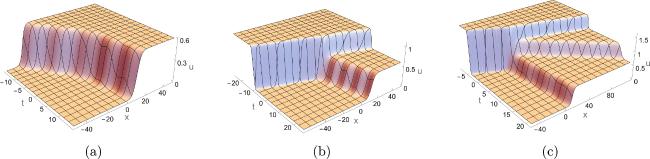
The following graphical illustrations give a good understanding of how those functions affect the propagation of solitary waves in nonuniform backgrounds by taking some special parameters and different choices of the coefficient functions b1(t), b2(t) by using Mathematica. Only consider taking α = 1 and plotting in the x, t plane. Figure 1 displays the standard shock waves in homogeneous backgrounds with b1(t) = 0, b2(t) = 0 and p1 = 0.6, p2 = 1.8, p3 = 1.1, d1 = 1, d2 = 1, d3 = 2, one shock wave in (a), interactions between two solitary waves in (b) and among three solitary waves in (c). Figure 2 displays the periodic shock waves in inhomogeneous backgrounds with ${b}_{1}(t)=4\sin t,{b}_{2}(t)=0$ and p1 = 0.6, p2 = 1.1, p3 = 1.6, d1 = 1, d2 = 1, d3 = 2, one shock wave in (a), interactions between two solitary waves in (b) and among three solitary waves in (c). Figure 3 displays the parabolic shock waves in inhomogeneous backgrounds with b1(t) = 0, b2(t) = t and p1 = 0.6, p2 = 1.1, p3 = 0.4, d1 = 1, d2 = 2, d3 = 1, one shock wave in (a), interactions between two solitary waves in (b) and among three solitary waves in (c). Figure 4 displays the mixed cases of periodic and parabolic shock waves in inhomogeneous backgrounds with ${b}_{1}(t)=4\sin t,{b}_{2}(t)=0.4t$ and p1 = 0.6, p2 = 1.1, p3 = 1.8, d1 = 1, d2 = 1.3, d3 = 1, one shock wave in (a), interactions between two solitary waves in (b) and among three solitary waves in (c). Figure 5 displays the mixed cases of periodic and shock waves in inhomogeneous backgrounds with p1 = 0.6, p2 = 1.1, p3 = 1.6, d1 = 1, d2 = 1, d3 = 2, one shock wave in (a), interactions between two solitary waves in (b) and among three solitary waves in (c). From those figures, it is easy to see that the influence of the coefficient functions b1(t), b2(t) on the waveform is very obvious, but does nothing about amplitude.
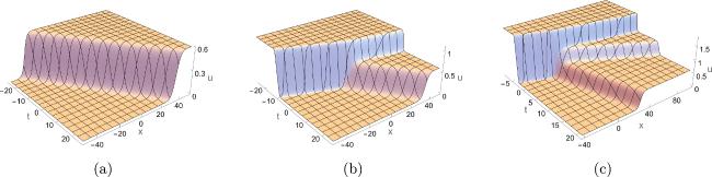
Figure 1. Standard shock waves in homogeneous backgrounds with b1(t) = 0, b2(t) = 0. |
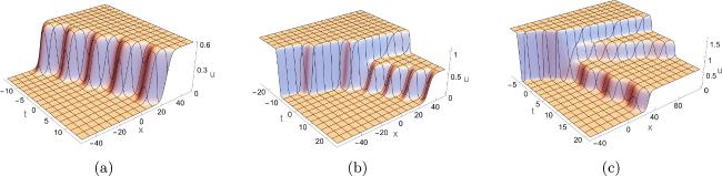
Figure 2. Periodic shock waves in inhomogeneous backgrounds with ${b}_{1}(t)=4\sin t,{b}_{2}(t)=0$. |

Figure 3. Parabolic shock waves in inhomogeneous backgrounds with b1(t) = 0, b2(t) = t. |
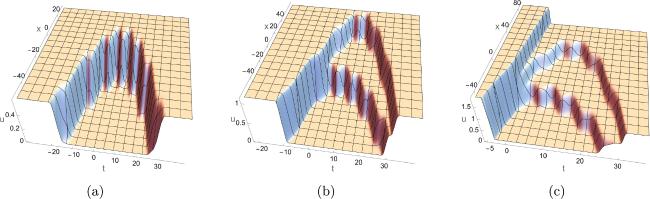
Figure 4. Mixed types of periodic and parabolic shock waves with ${b}_{1}(t)=4\sin t,{b}_{2}(t)=0.4t$. |
Figure 5. Mixed types of periodic and shock waves with ${b}_{1}(t)=\sin t,{b}_{2}(t)=\arctan t$. |