In the present article, we introduce a completely new regular model for static, spherically symmetric celestial fluid spheres in embedding class I spacetime. In this regard, needfully, we propose a new suitable metric potential eλ(r) to generate the present model. The various analyses on energy density, pressure, anisotropic factor, mass, compactness parameter, redshift, and energy condition make sure the model is physically viable on the ground of model stars Vela X-1, Cen X-3, SMC X-4, and LMC X-4. The reported solutions also respect the equilibrium state by satisfying the Tolman–Oppenheimer–Volkoff (TOV) equation and ensure stability by satisfying the causality condition, condition on the adiabatic index, and Harrison–Zeldovich–Novikov condition. The generated M − R graph matches the ranges of masses and radii for the model compact stars. Additionally, this study provides estimates of the moment of inertia based on the I − M graph.
Susmita Sarkar, Moumita Sarkar, Nayan Sarkar, Farook Rahaman. Relativistic model for anisotropic compact stars in embedding class-I spacetime[J]. Communications in Theoretical Physics, 2025, 77(1): 015403. DOI: 10.1088/1572-9494/ad7830
1. Introduction
Research on anisotropic compact stars has consistently remained an area of great interest in relativistic astrophysics after the pioneering work of Bowers and Liang [1]. Several comprehensive studies have elucidated our comprehension of highly dense spherically symmetric fluid spheres characterized by anisotropic pressure [2–5]. The pressure anisotropic can be found inside the celestial compact stars due to the formation of super-fluid neutrons [6], phase transition [7], pion-condensation [8], slow rotation [9], strong magnetic field [10], etc. Dev and Gleiser [11, 12] have explored the influences of pressure anisotropy on the mass, structure and physical properties of compact stars. Böhmer and Harko [13] demonstrated that anisotropic compact objects can exhibit much higher compactness compared to isotropic ones with their radii potentially approaching their corresponding Schwarzschild radii. Chaisi and Maharaj [14] developed an algorithm to find the anisotropic solutions of the field equations for anisotropic matter sources. Anisotropic compact stars have been also studied in the context of general relativity through the analytical approach [15–18] as well as the numerical approach [19–25]. Heintzmann and Hillebrandt [26] proposed a model for a relativistic, anisotropic neutron star at high densities and their analysis revealed that regardless of significant anisotropy, there is no upper limit to the mass of neutron stars. However, they noted that the maximum mass of a neutron star remains beyond 3-4 M⊙. Sharma et al [27] explored the theoretical feasibility of anisotropy within strange stars, which possess densities surpassing those of neutron stars yet falling short of black holes' densities. Alcock et al [28] and Haensel et al [29] introduced a comprehensive model for compact stars not composed of neutron matter, but characterized by exceedingly high densities within their interiors.
The maximum mass can be controlled by the brane tension λ which lies in the range 3.89 × 1036( ≡ 1.44M⊙) <λ < 1038dyne/cm2 concerning the equation of state (EoS). It is crucial to keep in mind that constructing exact interior solutions for non-uniform stellar configurations in the context of the braneworld is an exceedingly challenging task because of the nonlocality and non-closure of the braneworld equations [30]. The criteria for determining the restrictions needed on braneworld equations to achieve a closed system are still awaiting discovery [31]. To tackle this issue, it is essential to grasp the bulk geometry and comprehend how a 4-dimensional spacetime can be embedded. Castro et al [32] used the concept of embedding 4-dimensional spacetime in 5-dimensional hyperspace to embed a four-dimensional spacetime into a 5-dimensional braneworld. For the first time, Karmarkar [33] introduced a condition for embedding 4-dimensional spacetime into 5-dimensional Euclidean space in terms of the components of Riemannian curvature tensor, known as the embedding class-I spacetime. Randall–Sundrum model [34] is also based on our 4-dimensional spacetime being a hypersurface embedded into another 5-dimensional hypersurface in string theory. Ivanov [35] recently derived a condition akin to the Karmarkar condition for conformally flat spacetime. It is observed that the solutions arising from the two theories are entirely distinct. There are no physical solutions describing isotropic fluid distributions in the Karmarkar spacetime, i.e. class-I spacetime. However, viable physical solutions emerge when incorporating electric charge, anisotropy, or both [36–56].
In general relativity, an n-dimensional spacetime is classified as class-p if it is embedded in (n + p)-dimensional Pseudo Euclidean flat space. According to Kasner [56], the 4-dimensional spacetime of a spherically symmetric matter distribution can always be embedded in 6-dimensional Pseudo Euclidian space, which was also verified by Gupta and Goyel [57]. Eddington [58] discovered that an n-dimensional spacetime can always be embedded in k-dimensional Pseudo Euclidean space, where k = n(n + 1)/2 and the required minimum extra dimension to embedded is less than or equal to the number (k − n) or same as n(n − 1)/2. Particularly, the Schwarzschild interior solution is of class-I, the Schwarzschild exterior solution is of class-II, Friedman–Robertson–Lemaitre spacetime is of class-I [59–61] and the Kerr metric is of class-V [62].
In this article, we have introduced a new model for static, spherically symmetric anisotropic compact stars in the framework of embedding class-I spacetime based on the model compact stars, Vela X-1, Cen X-3, SMC X-4, and LMC X-4. Vela X-1 is a quintessential example of a high-mass x-ray binary (HMXB), comprising a neutron star orbiting closely around the 23.5 M⊙B0.5 Ib supergiant donor star HD 77 581. The rocket-borne experiment [63] and the Uhuru satellite observations [64] revealed the matter source was extremely variable. The comprehensive study of Vela X-1 is done in [65]. In 1967, the rocket-borne detector [63] discovered the compact star Cen X-3, which is the most luminous x-ray pulsar in our galaxy. Later, Giacconi et al [66] and Schreier et al [67] identified the binary and pulsar characteristics of Cen X-3 through satellite observations. Price et al [68] detected the compact star SMC X-4 residing in the Small Magellanic Cloud and it has significant variability in both the intensity and spectrum [69]. Schreier et al [70] reported the binary nature of SMC X-4 and discovered periodic occultations with an orbital period of around 3.9 days. For the first time, the compact star LMC X-4 was detected by the Uhuru satellite observations [64] in 1972. Later, Chevalier and Ilovaisky [71] revealed the binary nature of its optical counterpart.
The following article is structured as follows. We have formulated the Einstein field equations for static and spherically symmetric matter distribution in section 2. Section 3 describes the Embedding Class-I spacetime that meets the Karmarkar condition. We have introduced new class-I solutions along with mass, compactness parameter, surface redshift and gravitational redshift in section 4. Section 5 deals with the physical acceptance of the reported solutions. The matching condition of our internal solutions with the exterior Schwarzchild solution are analyzed section 6. We have analyzed the equilibrium and stability of the present model sections 7 and 8, respectively. The generating functions for our model have been computed in section 9. Section 10 describes the moment of inertia and mass relationship. Finally, the results and discussions have been conducted in section 11.
2. Einstein's field equations
To present the pertinent equations for characterizing a static, spherically symmetric self-gravitating locally bounded anisotropic fluids we consider the line element in Schwarzschild coordinate system (t, r, θ, φ) as [72]
where, eν(r) and eλ(r) are functions dependent solely on the radial coordinate r, referred to as metric potential functions. The energy-momentum tensor for the anisotropic fluid sphere can be expressed in the following form
where, ρ(r), Pr(r), and Pt(r) denote the energy density, radial pressure, and transverse pressure of the matter configuration, respectively. Uα is the four-velocity given by Uα = (e−ν(r)/2, 0, 0, 0) and χα is the unit space-like vector given by χα = (0, e−λ(r)/2, 0, 0), satisfying UαUα = − χαχα = 1, Uμχμ = 0. It is noted that
where, ‘′' stands for the derivative with respect to the radial coordinate r.
The anisotropic factor for static and spherically symmetric fluid configuration is characterized as Δ(r) = Pt(r) −Pr(r) [74], therefore, one can get the expression for Δ(r) from equations (5)–(6) as
Now, overall, we possess three field equations (4)–(6) for five unknown functions: eν(r), eλ(r), ρ(r), Pr(r), and Pt(r), therefore, we can freely select two of them so that the model becomes physically realistic.
3. The Karmarkar condition
In the study of stellar fluid configurations, the Karmarkar condition has a convenient effect because it creates a beautiful relationship between two metric potentials. In 1948, Karmarkar established a condition for embedding class-I spacetime in terms of the components of Riemannian curvature tensor Rαβγδ as [33]
The above condition is known as the Karmarkar condition, and by satisfying this, a 4-dimensional spacetime can be embedded in 5-dimensional flat space, i.e. becomes embedded in class-I spacetime. It is noted that the Karmarkar condition acts as the necessary condition only, Pandey and Sharma [75] derived the sufficient condition as R2323 ≠ 0.
For the line element (1), the non-zero components of Riemannian curvature tensor Rαβγδ are
It is noted that the pressure anisotropic Δ(r) becomes zero, i.e. it becomes isotropic for the following cases:
•
Case-1: $\displaystyle \frac{\lambda ^{\prime} (r)}{{{\rm{e}}}^{\lambda (r)}-1}=\displaystyle \frac{2}{r}$: in this case, one can get e−λ(r) = 1- Cr2 with C as an integration constant. Now, the condition (12) yields the other metric potential as ${{\rm{e}}}^{\nu (r)}={\left(A-B\sqrt{(1-{{Cr}}^{2})/C}\right)}^{2}$. On using e−λ(r) = 1- Cr2 in equation (4) one can see that the energy density becomes constant and this solution is essentially the Schwarzschild interior solution [77].
•
Case-2: $\displaystyle \frac{\nu ^{\prime} (r){{\rm{e}}}^{\nu (r)}}{2{{rB}}^{2}}=1$: in this case, one can obtain eν(r)=D + B2r2 with D as an integration constant. Similarly, the condition (12) yields eλ(r)=(D + 2B2r2)/(D + B2r2). This solution yields the Kohlar–Chao solution [78].
Here, we are interested in considering anisotropic pressure, therefore, we shall introduce a new metric potential function to generate the physical model.
4. New solutions via the Karmarkar condition
To formulate the model for anisotropic celestial matter configurations in embedding class-I spacetime, we introduce a completely new metric potential function as
For any physically viable anisotropic compact stars model, it is imperative to satisfy the following regularity and reality conditions consistently throughout the interior of the stellar configurations.
•
The spacetime must be devoid of singularities, meaning that the metric functions eλ(r) and eν(r) should remain finite and devoid of any singularities.
•
The energy density and radial pressure component ought to be positive and reach their maximum values at the centre while decreasing monotonically towards the boundary of the star. Furthermore, the radial and traversal pressures should be equal at the centre [4], indicating the absence of anisotropy at the centre of the star.
•
The mass function m(r) and compactness parameter u(r) must be positively finite and increasing in nature, also 2u(r) < 8/9, Buchdahl limit [80].
•
The surface redshift should be positively finite and increasing while the gravitational redshift should be positively finite and decreasing in nature.
•
The equation of state parameters for the stellar model must be ∈ (0, 1) [81]. Also, the stellar model needs to satisfy all the energy conditions [82, 83].
In order to properly justify our proposed model, we analyze the solutions graphically for four well-known compact stars, namely Vela X-1, Cen X-3, SMC X-4, and LMC X-4, and obtain the following results.
5.1. Evaluation of physical parameters
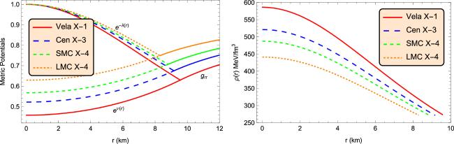
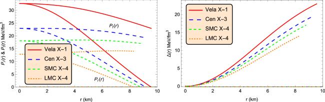
The introduced metric potentials e−λ(r) and eν(r), both are finite inside the compact stars (see figure 1 (left)), illustrating the non-singular geometry of the compact stars. Moreover, e−λ(r) and eν(r) are matched with the exterior Schwarzchild solution at the surfaces of the matter configurations as expected. The energy density is positive with the maximum value at the centres and decreases towards the surfaces, clear from figure 1 (right). The radial pressure Pr(r) is positively maximum at the centres and monotonically decreasing toward the surfaces of the stars with the zero values at the surfaces (see figure 2 (left)). The transverse pressure Pt(r) is also maximum at the centres of the stars and monotonically decreasing toward the surfaces of the compact stars Vela X-1 and Cen X-3 while it has slightly decreasing and increasing behaviours for the compact stars SMC X-4 and LMC X-4, clear figure 2 (left). Additionally, Pt(r) = Pr(r) at the centres of the stars and Pt(r) > Pr(r) for 0 < r ≤ R, which creates the positive anisotropy within the fluid configurations with the absence anisotropy at the centres (see figure 2 (right)). The symmetric profiles of energy density, radial pressure, and pressure anisotropic are depicted in figure 3, indicating the same satisfactory scenarios for all of them.
Figure 1. Characteristics of metric potentials (left) and energy density (right) against the radial coordinate r corresponding to the numerical values of constants given in table 1 for four well-known compact stars.
Figure 2. Characteristics of radial and transverse pressures (left) and anisotropic factor (right) against the radial coordinate r corresponding to numerical values of constants given in table 1 for four well-known compact stars.
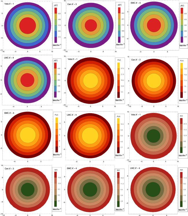
Figure 3. Symmetric profiles of energy density (red centres), radial pressure (yellow centres), and anisotropic factor (green centres) corresponding to numerical values of constants given in table 1 for four well-known compact stars.
Here, we obtain the central density and pressure at the centres of compact stars as
The above inequality is a boundary constraint on the constants A and B.
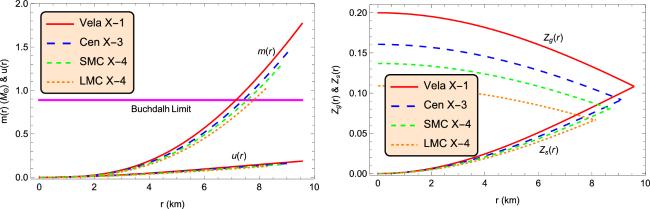
Furthermore, the mass function m(r) and compactness parameter u(r) for our proposed solutions are well-defined, zero at the centres of the fluid spheres and then positively increasing in nature within the compact stars with 2u(r) < 8/9, clear from figure 4 (left). Figure 4 (right) illustrates that the surface redshift is positively finite and increasing while the gravitational redshift is positively finite and decreasing in nature within the stars, moreover, at the surfaces (r = R) Z(R) =Zs(R) = Zg(R).
Figure 4. Characteristic of mass, compactness parameters (left) and surface, gravitational redshifts (right) against the radial coordinate r corresponding to numerical values of constants given in table 1 for four well-known compact stars.
5.2. Equation of state parameters
The EoS parameters ωr(r) and ωt(r) are dimensionless quantities that create the relationship between energy density and pressure. For our solutions, the EoS parameters ωr(r) and ωt(r) are obtained as [85, 86]
The behaviours of EoS parameters ωr(r) and ωt(r) are demonstrated in figure 5 (left), which indicates that both the parameters are within the region 0 < ωr(r), ωt(r) < 1 [81], and hence, the present solutions are fit to describe the physical matter configurations.
Figure 5. Characteristic of EoS parameters (left) and ρ(r) + Pr(r) (right) against the radial coordinate r corresponding to numerical values of constants given in table 1 for four well-known compact stars.
5.3. Energy conditions
The energy conditions are necessary to analyze the matter distribution (normal/exotic) inside the stellar objects. It is a well-established fact that physical mass distributions must adhere to all energy conditions within the matter configurations. The energy conditions, namely (i) null energy condition (NEC), (ii) weak energy condition (WEC) and (iii) strong energy condition (SEC) are defined as [82, 83]
Figures 5 (left)-6 along with figure 1 (right) make sure that the present solutions satisfy all the energy conditions, and hence, this result is again in favour of representing physical matter distribution inside the fluid configurations.
Figure 6. Characteristic of ρ(r) + Pt(r) (left) and ρ(r) + Pr(r) + 2Pt(r) (right) against the radial coordinate r corresponding to numerical values of constants given in table 1 for four well-known compact stars.
6. Matching of interior and exterior solutions
In the stellar model, the interior solution will be matched with the exterior Schwarzschild solution at the surface r = R of the star [77]. Indeed, the matching of interior and exterior solutions helps to determine the values of constants involved in the interior solution. The Schwarzschild exterior solution is given as [77]
Here, b and c are free parameters to derive well-behaved solutions. Also, the mass M and radius R will be selected accordingly for different stars.
7. Equilibrium analysis
In this section, we will examine the equilibrium of the fluid distributions described by our solutions. For an anisotropic fluid sphere, the gravitational force, hydrostatic force, and anisotropic force together create the equilibrium situation, and this situation can be described by the Tolman–Oppenheimer–Volkoff (TOV) equation. The generalized TOV equation for anisotropic fluid distribution can be written as [86, 87]
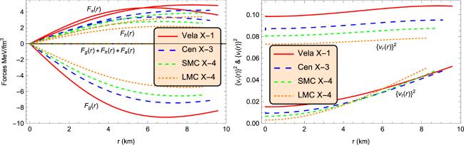
where, ${F}_{g}(r)=-\tfrac{1}{2}\nu ^{\prime} (r)\{\rho (r)+{P}_{r}(r)\}$ is termed as the gravitational force, Fh(r) = − dPr(r)/dr is termed as the hydrostatic force, and Fa(r) = 2Δ(r)/r is termed as the anisotropic force.
For the present solutions, the three distinct forces are derived in the following expressions
We illustrate the behaviours of these three forces graphically in figure 7 (left), indicating that our solutions depicting fluid configurations are in states of equilibrium.
Figure 7. Characteristics of different forces (left) and radial, transverse velocities of sound (right) against the radial coordinate r corresponding to numerical values of constants given in table 1 for four well-known compact stars.
8. Stability analysis
The analysis of stability is very crucial in evaluating the viability and consistency of the model of stellar objects. Indeed, the celestial objects that demonstrate stability against external perturbations are particularly intriguing to study. Here, we explore the stability of the model through (i) Causality condition along with stability factor, (ii) Adiabatic index, and (iii) Harrison–Zeldovich–Novikov criterion.
8.1. Causality condition
According to general relativity, nothing can travel faster than light, i.e. the velocity of light is the maximum velocity that ever exists, which is considered to be equal to 1 in the gravitational unit. The causality condition states that the radial velocity vr(r) and transverse velocity vt(r) of sound within the physical fluid distribution must be less than the velocity of light, mathematically, 0 ≤ vr(r), vt(r) < 1 [89]. Now, vr(r) and vt(r) inside the anisotropic compact star are defined as
Figure 7 (right) reveals that the present model nicely holds the causality condition, i.e. our model represents physically realistic fluid configurations. Taking into account the concept of cracking of Herrera [90], Abreu et al [91] introduced the stability conditions for the stellar model concerning the stability factor ${S}_{F}(r)=\left[{\{{v}_{t}(r)\}}^{2}-{\{{v}_{r}(r)\}}^{2}\right]$ as: the matter configuration is potentially stable if −1 < SF(r) < 0 and unstable if 0 < SF(r) < 1. Figure 8 (left) indicates that the present solutions depicted matter configurations are potentially stable.
Figure 8. Characteristics of stability factor (left) and adiabatic index (right) against the radial coordinate r corresponding to numerical values of constants given in table 1 for four well-known compact stars.
8.2. Adiabatic index
The relativistic adiabatic index serves as a crucial factor in analyzing the stability of stellar fluid spheres by quantifying the change in pressure as the matter density undergoes slight variations. The relativistic adiabatic index Γr(r) is defined as [92]
According to Bondi [92], the stellar Newtonian sphere will be stable if the adiabatic index Γr(r) > 4/3 and Γr(r) = 4/3 represents the state of neutral equilibrium. Figure 8 (right) shows that the present solutions recommended adiabatic index Γr(r) > 4/3, which adds another feather in favour of stable fluid configurations.
8.3. Harrison–Zeldovich–Novikov criterion
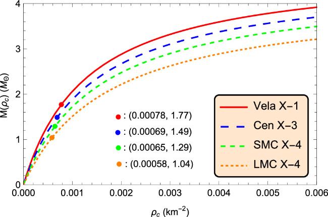
According to Harrison–Zeldovich–Novikov [84, 93], the mass should increase with the increase of central density ρc for the static stability state of fluid configurations, mathematically, ∂M(ρc)/∂ρc > 0 for the static stability state. The mass as a function of the central density is obtained as
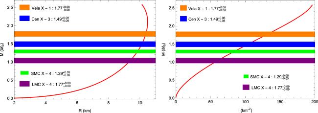
The present solutions satisfy the static stability criterion and thus remain stable, clear from figure 9. Also, we display the mass-surface profile in figure 10 (left), illustrating that the ranges of masses and radii are very close to the observed values.
Figure 9. Characteristics of mass against the central density ρc corresponding to numerical values of constants given in table 1 for four well-known compact stars.
Figure 10. Characteristics of mass M against the surface radius R (left) and mass M against the moment of inertia I (right).
9. Generating functions
In 2008, Herrera [94] devised an algorithm utilizing generating functions to derive all feasible anisotropic solutions of Einstein's field equations as
Bejger and Haensel [95] employed a technique wherein a static solution could transition into a rotating one by utilizing an approximate expression for the moment of inertia I given as
The profile of I against mass M is demonstrated in figure 10 (right), which helps to predict the possible approximate moment of inertia against observed ranges of masses.
11. Result and discussions
In this article, we have introduced a new model for static, spherically symmetric anisotropic compact stars in the framework of embedding class-I spacetime. The present solutions are analyzed based on the four well-known compact stars, namely Vela X-1, Cen X-3, SMC X-4, and LMC X-4, and coherently we have found the following key results.
The proposed metric potentials are non-singular inside the compact stars with eλ(0)=1 and ${{\rm{e}}}^{\nu (0)}\,={\left[A+\sqrt{a}B\mathrm{log}[\sinh (c)]/2b\right]}^{2}$ = positive constant, ensuring that the metric potentials are physically fit to generate the physically viable stellar model (see figure 1 (left)).
The energy density and pressures are positively finite throughout the interior of fluid spheres having maximum values at the centers of the fluid spheres, clear from figures 1 (right) and 2 (left). In addition, Pr(R) = 0, Pr(0) = Pt(0), and Pt(r) > Pr(r) for 0 < r ≤ R (see figure 2 (left)), these results ensure that the pressure anisotropic is positive for 0 < r ≤ R and vanishes at the centre (see figure 2 (right)). Indeed, the positive pressure anisotropic creates a repulsive anisotropic force that can assist in constructing a more stable compact star [96]. The symmetric profiles of energy density, radial pressure, and pressure anisotropic have ensured their desired characteristics (see figure 3). The numerical values of central, surface densities and central pressure for the model compact stars are provided in table 2. Interestingly, the central and surface densities both are of order 1014 gm cm−3, and the central pressure is of order 1034 gm cm−2, these respect the observational data.
The mass m(r) and compactness parameter u(r) are zero at the centres of the stars, after that, monotonically increasing toward the surfaces, clear form figure 4 (left). Buchdahl [80] proposed a clear prediction regarding the maximum attainable mass for relativistic stars as M < 4R/9, or equivalently $2u(R)\lt \tfrac{8}{9}$, this is respected by our solutions (figure 4 (left) and table 2).
The surface redshift Zs(r) approaches zero at the centres and then steadily increases towards the surfaces of the model spheres. Conversely, the gravitational redshift Zg(r) exhibits an inverse pattern, reaching its peak at the centres and declining towards the surfaces of the fluid configurations (see figure 4 (right)). Moreover, Zs(r) and Zg(r) meet together at the surfaces, i.e. Z(R) = Zs(R) = Zg(R). The numerical results for Z(R) given in table 2 respect the range provided by Ivanov [4].
The EoS parameters for the present solutions are nicely fitted in the range 0 < ωr(r), ωt(r) < 1 [81] (see figure 5 (left)). Also, the solutions satisfied all the energy conditions, clear from figures 5 (right)–6 along with figures 1 (right). In this context, one can say that our solutions presenting matter configurations are physical.
The model compact stars are in equilibrium positions under the simultaneous action of gravitational, hydrostatic, and anisotropic forces. Indeed, hydrostatic, and anisotropic forces act as repulsive forces to balance the attractive gravitational force, this scenario is clear in figure 7 (left).
The stability of the model is analyzed through the causality condition, adiabatic index, and Harrison–Zeldovich–Novikov criterion. The sound velocities vr(r) and vr(r) are positive and less than one (speed of light) (see figure 7 (right)), moreover, the stability factor SF(r) is negative (see figure 8 (left)), indicating that the solutions represent physically stable matter distributions. Furthermore, the profiles of the adiabatic index (see figure 8 (right)) and mass in terms of central density (see figure 9) also respect the stable scenario of the model fluid configurations. Figure 9 also suggests that the central densities of the model stars are, Vela X-1: 0.000 78 /km2, Cen X-3: 0.000 69/km2, SMc X-4: 0.000 65/km2, and LMC X-4: 0.000 58/km2.
The mass-surface radius profile describes the same ranges of masses and radii as given in table 1, i.e. our solutions providing mass and radius ranges are closely matched with the observed values (see figure 10 (left)). In addition, the corresponding moment of inertia I can be deduced from the I − M graph, figure 10 (right) as for Vela X-1: I ≈ 1.483 × 1045 g cm2; Cen X-3: I ≈ 1.178 × 1045 g cm2, SMC X-4: I ≈ 0.897 × 1045 g cm2, and LMC X-4: I ≈ 0.692 × 1045 g cm2.
Table 1. Numerical values of masses, radii, and constants a A, B for four well-known celestial compact stars corresponding to b = 0.0001 /km2 and c = 1.
It is noted that the physical parameters in this model have followed the same desired behaviours as described in [36–38, 46, 98–107]. Moreover, our obtained numerical results of the physical parameters given in table 2 are very close to the results provided by [39, 48, 108–110] with the values of moment of inertia I in order of 1045 g cm2 [44, 97, 111]. Therefore, all these behaviours enrich our model for physical acceptability.
Table 2. Numerical values of the central and surface densities, average density ρav = 3M/4πR3, central pressure, surface redshift at the boundary, twice of compactness parameter with buchdahl limit, and moment of inertia for four celestial compact stars mentioned in table 1.
Finally, all the significant results ensure that the present model is physically well-behaved and suitable to describe the static, spherically symmetric stable anisotropic compact stars in the framework of embedding class-I spacetime.
FR would like to thank the authorities of the Inter-University Centre for Astronomy and Astrophysics, Pune, India for providing research facilities. We are thankful to the reviewers for their constructive suggestions.
HerreraL, Di PriscoA, MartinJ, OspinoJ, SantosN O, TroconisO2004 Spherically symmetric dissipative anisotropic fluids: a general study Phys. Rev. D69 084026
SilvaH O, MacedoC F B, BertiE, CrispinoL C B2015 Slowly rotating anisotropic neutron stars in general relativity and scalar-tensor theory Class. Quantum Gravity32 145008
ThakadiyilS, JasimM K2013 Invariant solutions of Einstein's field equations for conformally flat fluid spheres of embedding class one Int. J. Theor. Phys.52 3960
GuptaY K, GoelM P1975 Class two analogue of TY Thomas's theorem and different types of embeddings of static spherically symmetric space-times Gen. Rel. Grav.6 499
LemaîtreG1927 Un Univers homogène de masse constante et de rayon croissant rendant compte de la vitesse radiale des nébuleuses extra-galactiques Ann. Soc. Sci. Bruxelles, Ser.47 49
62
KuzeevR R1980 Inmersion class of a Kerr field Gravit. Teor. Otnosit.16 93
63
ChodilG1967 X-ray intensities and spectra from several cosmic sources Astrophys. J.150 57
SchreieE, LevinsonR, GurskyH, KellogE, TananbaumH, GiacconiR1972 Evidence for the Binary Nature of Centaurus X-3 from UHURU X-Ray Observations Astrophys. J.172 79
ChevalierC, IlovaiskyS A1977 The binary nature of the LMC X-4 optical candida Astron. Astrophys.59 L9
72
StephaniH, KramerD, MaccallumM, HoenselaersC, HelrtE2003Exact Solutions of Einstein Field Equations Monographs on Mathematical Physics 2nd edn Cambridge Cambridge University Press
73
BondiH1964 Massive spheres in general relativity Proc. Roy. Soc. Lond. A282 303 317
MauryaS K, GuptaY K, RayS, ChowdhuryS R Spherically symmetric electromagnetic mass models of embedding class one arXiv:1506.02498
77
SchwarzschildK1916 Über das Gravitationsfeld einer Kugel aus inkompressibler Flüssigkeit nach der Einsteinschen Theorie Sitz. Deut. Akad. Winn. Math-Phys. Berlin24 424
78
KohlerM, ChaoK L1965 Zentralsymmetrische statische Schwerefelder mit Räumen der Klasse 1 Z. Naturforsch. Ser. A20 1537
RahamanF, RayS, JafryA K, ChakrabortyK2010 Singularity-free solutions for anisotropic charged fluids with Chaplygin equation of state Phys. Rev. D82 104055
RawlsM L, OroszJ A, McClintockJ E, TorresM A P, BailynC D, BuxtonM M2011 Refined neutron star mass determinations for six eclipsing x-ray pulsar binaries Astrophys. J.730 25
SinghK, BharP, PantN2016 A new solution of embedding class I representing anisotropic fluid sphere in general relativity Int. J. Mod. Phys. D25 1650099
JasimM K, MauryaS K, Al-SawaiiA S M2020 A generalised embedding class one static solution describing anisotropic fluid sphere Astrophys. Space Sci.365 9
SatyanarayanaG, BishtR K, PantN2020 Relativistic modelling of stellar objects using embedded class one spacetime continuum Mod. Phys. Lett. A35 2050097


